a^2 + b^2 = c^2

Overview

In this project we build a raytracer which lets us render scenes. The first step consisted of generating rays that shoot from the camera through the image plane and into the scene. In later parts of the project we figured out how those rays bounce through the scence and how lighting and reflectance changes as a result of different surfaces. We also implemented triangle and sphere intersection methods that allow us to render scenes. The final step was adding global illumination that allows us to simulate rays bouncing off multiple objects, which allowed us to generate more realistic renderings.

Part 1: Ray Generation and Scene Intersection (20 Points)

Walk through the ray generation and primitive intersection parts of the rendering pipeline.

Ray generation begins with converting normalized image space coordinates (0 to 1 range) to a coordinate in the camera space of the form (x,y,-1). This is done with a shift and scale operation. Next we convert from camera space coordinates to world space coordinates by using the global translations and the camera to world rotation matrix. When rendering a scene we cast multiple rays through each pixel and average over those rays to determine a pixel color value.

Explain the triangle intersection algorithm you implemented in your own words.

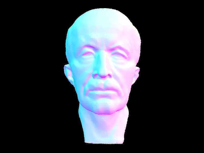
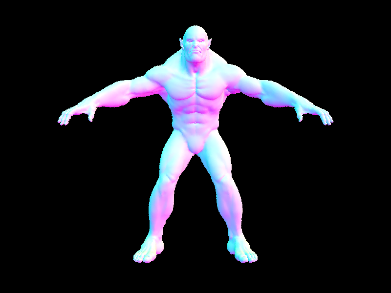
The first step is determining the t value for which the ray will intersect with the plane that contains the triangle of interest. This is done by setting up a system with the equation of the plane and of the ray. Given an intersecting t value we can compute a location on the plane where the ray intersects. We compute the barycentric coordinates for this point (using the Moller Trumbore algorithm) and check that alpha, beta, gamma are between 0 and 1 to determine if it's in the triangle. We also compute the normal at the intersection point by interpolating between the vertex normals using the barycentric coordinates.

Show images with normal shading for a few small .dae files.

Part 2: Bounding Volume Hierarchy (20 Points)

Walk through your BVH construction algorithm. Explain the heuristic you chose for picking the splitting point.

We construct the BVH by first taking all bounding boxes and merging them together for all primitives for the current node we are constructing. We compute 3 candidate split points along the center point of the x, y, and z directions of the merged bounding box. We then determine how many primitives will go on the left and the right of the split point for each axis. To determine the best axis to split on we compute the entropy of the split based on the proportion of primitives on each side and pick the axis that has the largest entropy (the most equal split between the left and right sides to keep the tree balanced). We then recursively perform this splitting process on the left and right sides of the tree until we reach the leaf nodes.

Show images with normal shading for a few large .dae files that you can only render with BVH acceleration.

Compare rendering times on a few scenes with moderately complex geometries with and without BVH acceleration. Present your results in a one-paragraph analysis.

For the cow, it took 39s without BVH acceleration, and 2.0976s with BVH acceleration. Similarly, the teapot took 17.7s and 0.4638s without, and the beetle took 39.7s with and 0.3905s without. BVH acceleration helps with rendering the images faster because each ray traverses the tree of boxes, making it log(N) time instead of O(N).

Part 3: Direct Illumination (20 Points)

Walk through both implementations of the direct lighting function.

In estimate_direct_lighting_hemisphere, we implemented the monte carlo estimator described in lecture. We generated N number of random rays with directions sampled from the hemisphereSampler. Each of these rays originated from hit point and in a random direction in the world frame. If these rays intersected the bvh, we get the emission from that new intersection point and the reflectance of the original intersection. This combined with cos(wi) and the pdf (1/2PI because it's a hemisphere) gives us the information needed to calculate the outgoing light from each ray. We then averaged it with the number of samples to estimate how much light arrived at that intersection point from elsewhere.

In estimate_direct_lighting_importance, we implemented a sampling function that samples rays coming from light sources rather than uniformly across a hemisphere. There are two cases: 1) If we are sampling point light, then there is only one potential direction to sample (from the hit point to the position of the point light) and 2) if we are sampling a different light source we using the sampling function from that light to determine a ray. We then send a ray from the hit point in the direction of the sampled light. If the ray intersects a scene object before hitting the light, then we don't add the light from the source onto the hit point. If there is no collision then we add the illuminance from the light source according to the reflectance equation.

Show some images rendered with both implementations of the direct lighting function.

Focus on one particular scene with at least one area light and compare the noise levels in soft shadows when rendering with 1, 4, 16, and 64 light rays (the -l flag) and with 1 sample per pixel (the -s flag) using light sampling, not uniform hemisphere sampling.

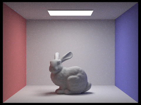
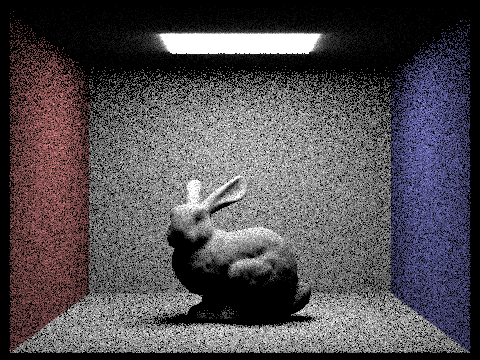
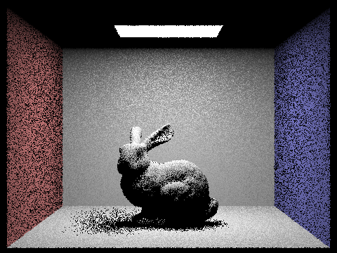
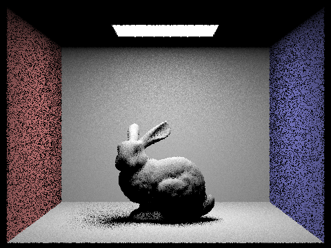
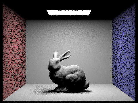
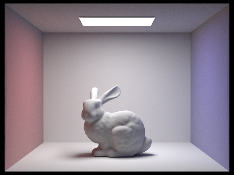
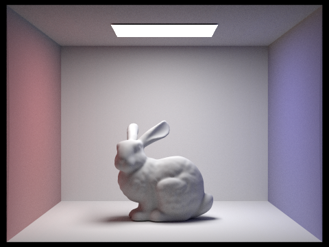
With a higher number of samples per light ray the noise on the bunny dramatically reduces. This is because when we sample more times along the area light in the scene we are more likely to get a accuracy average of the illuminance at each point on the bunny.

Compare the results between uniform hemisphere sampling and lighting sampling in a one-paragraph analysis.

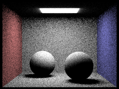
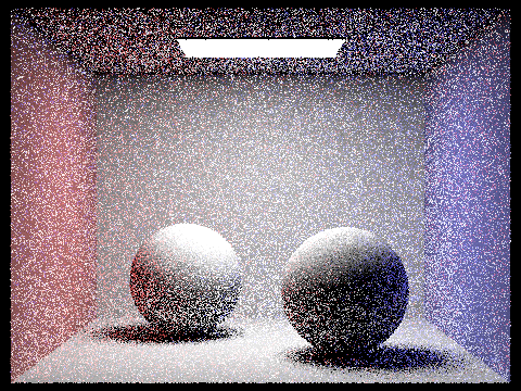
Importance sampling heavily reduced the amount of noise as seen in the CBbunny and CBspheres example. This is generating rays in the direction of more received light is a lot more efficient than generating completely random rays in a hemisphere. Because these are single bounce examples, we only care about rays that produce light and not the ones from the walls. Especially in scenes like these where the light is particularly small surrounded by black walls, importance sampling will have a larger effect than uniform sampling.

Part 4: Global Illumination (20 Points)

Walk through your implementation of the indirect lighting function.

We always start with one bounce (using our estimate_direct_lighting_importance function). We then recursively keep on bouncing that ray until it, misses (i.e. doesn't hit a light), reaches the maximum ray depth, or the russian roulette termination probability gets hit. If none of the listed cases are true, that means the ray hit something and we can continue. At every point where the ray hits something, we add onto our summed radiance from all the bounces.

Show some images rendered with global (direct and indirect) illumination. Use 1024 samples per pixel.

Pick one scene and compare rendered views first with only direct illumination, then only indirect illumination. Use 1024 samples per pixel. (You will have to edit PathTracer::at_least_one_bounce_radiance(...) in your code to generate these views.)

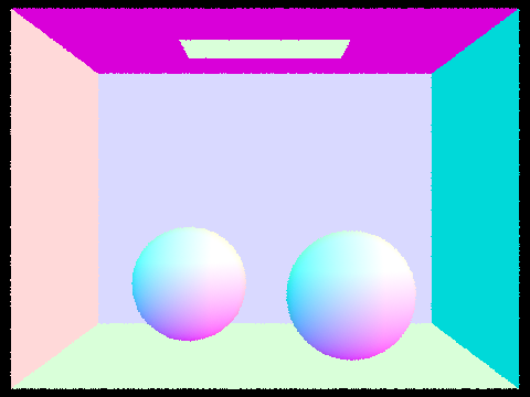
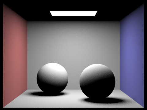
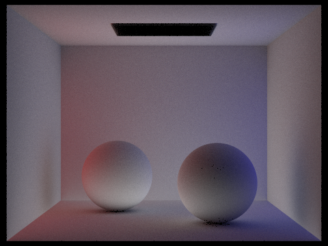
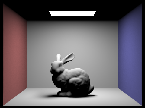
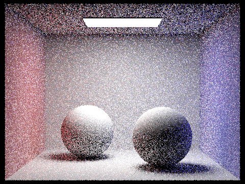
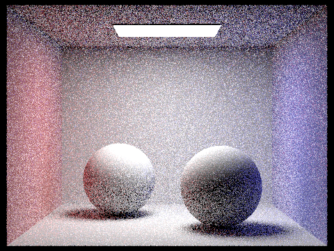
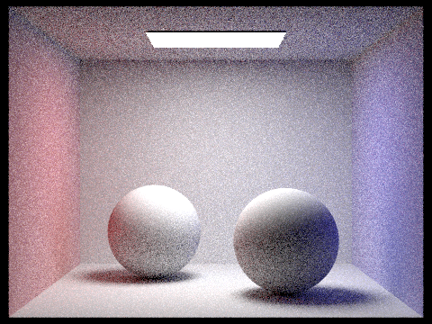
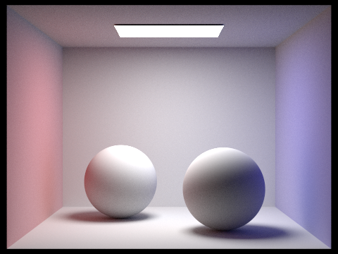
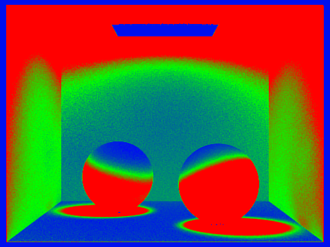
When using only direct illumination we are considering zero bounces and one bounce. When using indirect illumination, we are using neither zero or one bounce, but only two bounce illumination. In the indirect lighting example we see that the area light source is not illumination (since no zero bounce illumination), but we do see the colors from the walls reflected onto the spheres. With the direct lighting since there is no two bounce illuminations we don't have the red and blue colors from the walls showing up on the spheres.

For CBbunny.dae, compare rendered views with max_ray_depth set to 0, 1, 2, 3, and 100 (the -m flag). Use 1024 samples per pixel.

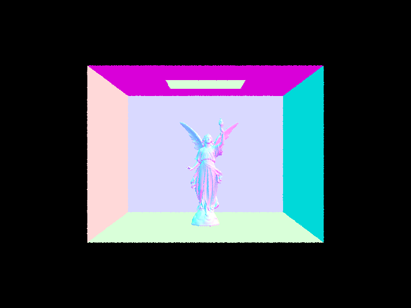
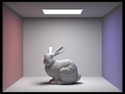
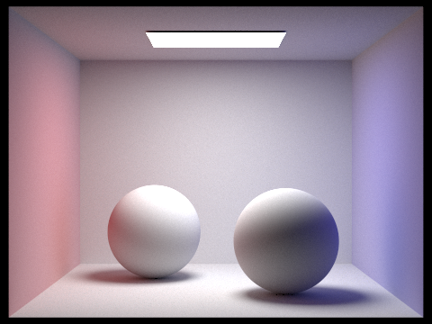
As we increase the m parameter, we have every randomly generated ray continue bouncing around the scene until we terminate, gathering more light everywhere. This makes the overall generated scene appear brighter and more illuminated. A notable feature in the bunny is that the ceiling instantly brightens after increasing the max_ray_depth by just 1 because the rays are able to bounce towards the top of the image instead of instantly stopping once it arrives on the bunny or the walls.

Pick one scene and compare rendered views with various sample-per-pixel rates, including at least 1, 2, 4, 8, 16, 64, and 1024. Use 4 light rays.

As we increase the sample rate per pixel, the images get less noisy and the pixels get less variance since we're shooting more rays per pixel.

Part 5: Adaptive Sampling (20 Points)

Explain adaptive sampling. Walk through your implementation of the adaptive sampling.

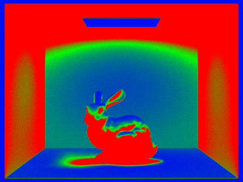
In adaptive sampling, we rewrote the raytrace_pixel function to take into account how many samples we have taken so far rather than always going through ns_aa number of samples. Following the algorithm described in the spec, we defined variables for the s1, s2, mean, and SD to occasionally check (every samplesPerBatch times) whether we reached the termination condition (maxTolerance * mean). Once we've crossed that threshold, we stop sampling this particular pixel. This ensures that we only sample a large amount of times in more complicated parts of the scene. For example, the bunny is more complicated than most of the wall which is why we can see the bunny is more red than the walls in the sample rate image.

Pick two scenes and render them with at least 2048 samples per pixel. Show a good sampling rate image with clearly visible differences in sampling rate over various regions and pixels. Include both your sample rate image, which shows your how your adaptive sampling changes depending on which part of the image you are rendering, and your noise-free rendered result. Use 1 sample per light and at least 5 for max ray depth.