Assignment 3: PathTracer

Overview

For project 3-1, we implemented ray and scene generation, bounding volume hierarchies, direct illumination, global illumination, and adaptive sampling to create images of realistic looking objects affected by light sources. We really enjoyed the process of being able to incorporate concepts from class such as russian roulette into practice. Overall it was a great experience being able to see our images come to life.

Part 1: Ray Generation and Intersection

For part 1, we implemented the ray generation and primitive intersection parts of the rendering pipeline. Ray generation generates Ray objects while primitive intersection uses Rays to test whether a Ray intersects with a primitive object if so, tells us the nearest time of intersection.

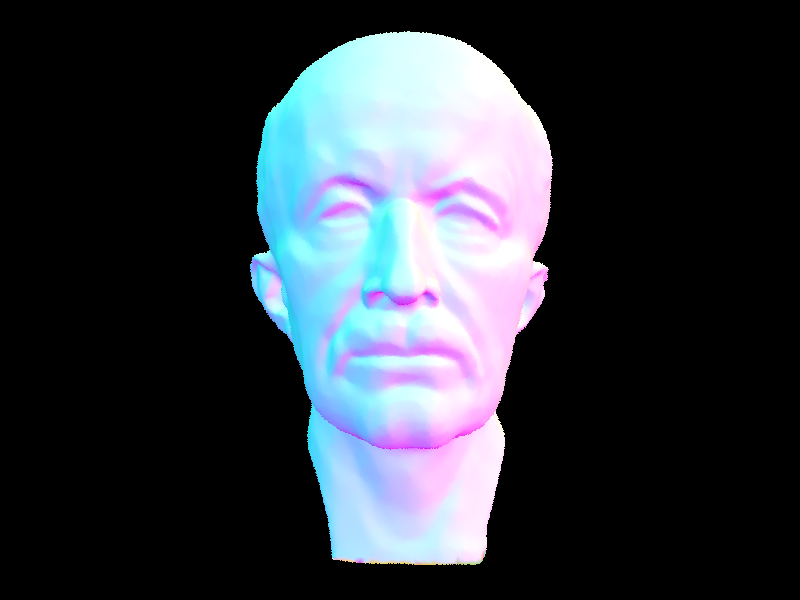
For part 1.1, we implemented Camera::generate_ray(...). The purpose of this function is to turn an image coordinate into a Ray in world space. To achieve this, we start by using proportions to transform the image space coordinate to camera space. We then multiply this camera space coordinate by the given camera to the world space vector in order to get our world space direction. From here, we normalize the direction and then construct a Ray using this direction and the given camera position as the starting point for our Ray. We then set our max_t value to nClip and our min_t value to fClip and return our Ray. This part took us a long time to figure out since initially, we initially were not normalizing correctly. We solved it by realizing that the norm function doesn't return the normalized vector but the Euclidean length.

For part 1.2 we implemented PathTracer::raytrace_pixel(...), which uses Monte Carlo estimation in order to estimate the value of each pixel in our scene. It works using a loop which randomly samples a pixel from image space, generating a ray from that pixel, estimating the radiance of that ray, and then returning the average of the radiance values. Initially our function didn't work due to floating point errors which we found after our print statements revealed certain values to evaluate to 0 when they weren't supposed to.

For part 1.3, we implemented triangle intersection by first using the Moller Trumbore algorithm, which gave us a vector containing t, b₁, and b₂ by using matrix math on the vertex coordinates of the triangle and the ray origin and direction. Using these values we checked them to see if the Ray intersected the triangle by checking if t fell between the Ray's max_t and min_t values (the Ray's constraints), and if b₁, b₂, and b₃ (which evaluated to 1 - b₁ - b₂) were all between 0 and 1 (to ensure a valid intersection). If these conditions were satisfied, it meant that the Ray interested the Triangle, so we updated the Ray's max_t to the t returned from the Moller Trumbore algorithm (to ensure the ray doesn't go through the object) and updated isect's (the Intersection object's) t value with the correct time of intersection, n value with the interpolation of the triangle's vertex normals (n1, n2, and n3) with b₁, b₂, and b₃, it's primitive value to the Triangle object, and it's bdsf to the Triangle's bdsf. When working on this part, we encountered a bug where we had a strange image that wasn't the correct rendering for CBempty. We tried debugging on our own but ended up getting help from a TA. We learned that we didn't implement the Moller Trumbore algorithm correctly and were multiplying instead of getting the dot product. We also didn't set the Ray's max_t which wasn't updating the Ray and resulted in the wrong rendering of the image.

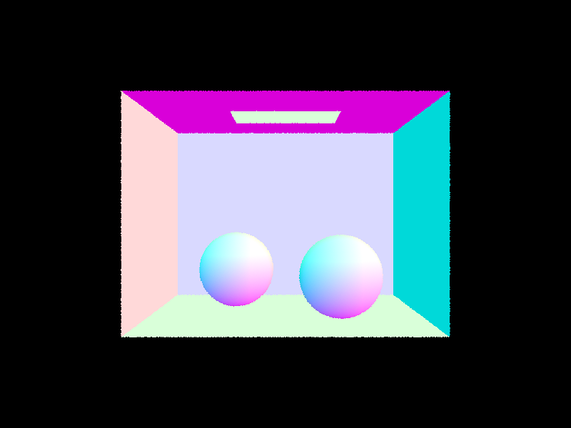
For part 1.4, we implemented sphere intersection. We pulled the origin and the radius of the Sphere as well as the origin o and direction d of the Ray. Using this information we found a = dot(d, d), b = dot(2 * (o - origin), d), and c = dot((o - origin), (o - origin)) - radius^2 (essentially using the formula of a circle to sphere to check for ray intersection). We were able to use the quadratic formula to find the new_t value and then check if it was inside of the Ray's max_t and min_t. If it was inside these values, we updated the Ray's max_t and the Intersection's t with the new_t, primitive with the sphere given to us, bsdf with the sphere's bsdf, and n to the normal(o + d * new_t).

Part 2: Bounding Value Hierarchy

In part 2.1, we implemented BVHAccel:construct_bvh(...) by first creating a BBox called bbox to populate. We then iterated through all primitives and expanded bbox to include the primitive's bounding box. Afterwards, we created a BVHNode called node using bbox. We checked our base case, which is if the amount of primitives inputted was less than or equal to the max_leaf_size, and if it was, we updated node's start and end to be the same as the ones inputted and returned node. Otherwise, if our base case isn't satisfied, we sort our primitives using the value of the longest axis (determined by the largest value in the extent instance of bbox) of their centroids. We use the median of these sorted primitives as our splitting point. Then we called construct_bvh for the left and right leaves of node (with half the sorted primitives passed to the left and the other passed to the right) to recurse through and create a tree structure.

In part 2.2, we implement BBox::intersect(...) which returns whether a Ray intersects a BBox within the time ranges of t0 and t1. In order to do this we implement ray-plane intersection, basically seeing how the ray intersects with each axis of a plane and then combining the results to see if the times of each axis intersection match a valid plane intersection. In other words, we check that the latest time a ray enters an axis is less than the earliest time a ray enters an intersection to ensure a valid intersection. If a valid intersection occurs, we update t0 and t1 to the new intersection times. We had a lot of issues with this part due to our initial lack of conceptual understanding on how to use the values of the axis intersections. We solved this issue by consulting TAs in office hours and rewriting our solution several times.

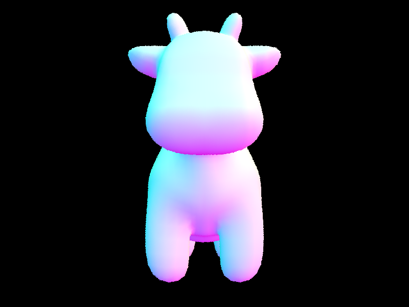
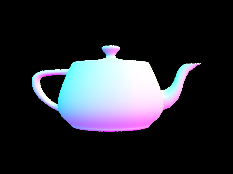
In part 2.3, we implement BVHAccel::has_intersection(...) and BVHAccel::intersect(...) which detect an intersection between a ray and a BVH object. In intersect we first check to see if the ray intersects the given BBox. If not we immediately return false. If so, we update the ray's min_t and max_t with the outputs of BBox::intersect(...). We then check our base case (whether our given BVH node is a leaf). If it is, we check for an intersection between the ray and each primitive in the node while updating our given Intersection object if an intersection occurs. If no intersection occurs, we return false, otherwise we return true. If our base case is not satisfied, we call BVHAccel::intersect(...) on the left and right values of the node and return if either outputs true. Due to the nature of our functions, passing the original Intersection object into both these recursive calls will result in the correct Intersection object outputted. Initially, I made a simple indexing error when I was trying to split the primitives. This resulted in me leaving out a primitive with each function call. I resolved it by seeing that there were black faces in the cow in the GUI and checking my partitioning.

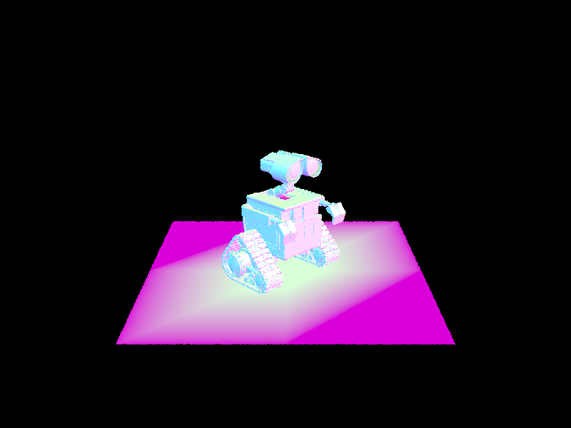
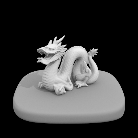
Rendering without BVH acceleration takes longer compared to rendering with BVH acceleration. Rendering images with BVH acceleration takes images like the cow 0.0402 seconds and the teapot takes 0.0930 seconds which is less than one second. This is a significant decrease in time compared to rendering without BVH acceleration which takes the cow 18.2732 seconds and the teapot 9.7807 seconds. This difference in rendering time is obvious in images like the banana that takes 37.5120 seconds without BVH acceleration and takes 0.2790 seconds with it. Before implementing BVH acceleration, the entire scene was traversed even if there were no intersections, however using BVH acceleration only uses the nodes that are guaranteed to interest and discards the nodes that don't intersect. This significantly decreases rendering time because we only look at the nodes that we want and need instead of looking at everything. BVH significantly improves results because it eliminates the need to iterate through every object and efficiently identifies the range of objects which could have been intersected.

Part 3: Direct Illumination

For 3.1, we implemented DiffuseBSDF::f where we use the concept of irradiance falloff to return the reflectance given wi and wo within the hemisphere.

For 3.2, we implemented zero_bounce_radiance which returns the emission of the object intersected by the given ray. We also had to update est_radiance_global_illumination to return zero bounce instead of normal shading. In this part, we ran into an issue where only a black image would render since we had a floating point error in raytrace_pixel from part1. We fixed it by converting the correct value to a float.

For part 3.2, we implemented estimate_direct_lighting_hemisphere (direct lighting with uniform hemisphere sampling) by using a Monte Carlo estimator with num_samples to find the radiance at an intersection. For each sample, we get wj, a random direction within the hemisphere, by using the given hemisphereSampler. We get f_val by calling f of the bsdf on w_out and wj to get the reflectance of the intersected object. We set pdf to 1/(2 * pi) due to it being in a hemisphere. We then create a Ray r_j using w_j converted to world space (we convert w_j to world space by multiplying it with the given object to world matrix)(we need to convert this direction to world space since Rays operate in world space while bsdf operate in object space) and an origin of hit_p. We set r_j's min_t to be EPS_F to avoid the ray returning an intersection at the hit point. We then checked if r_j intersects an object within our BVH and we add (f_val * li_val * cos_val) / p_val to our summation vector L_out. li_val is the emission of the original intersection, cos_val was the dot product of the normal with wj, and p_val is pdf from sample_f. After iterating through all of the samples, we averaged the sum vector L_out by the number of samples and returned the resulting vector. Initially, our rendering didn't work since we mistook the cos_val to be the dot product of the normal with li_val. It wasn't until we consulted a fellow student who corrected our conceptual misunderstanding that we found the error.

For part 3.4, we implemented estimate_direct_lighting_importance (direct lighting by importance sampling) by using a Monte Carlo estimator which iterates through the lights in the scene to find the radiance at an intersection. We also iterate through each light ns_area_light times in order to be able to take in multiple samples at each light. In each iteration, we get li_val by calling sample_L on the current light and hit_p. By calling this function we also get wi, the world-space direction between hit_p and the light source, the distance from hit_p to the light source, and a pdf. We then create Ray r_wi with an origin of hit_p and a direction of wi. We set r_wi's min_t to be EPS_F (for the same reasons as 3.3) and its max_t to be dist_to_light - EPS_F (in avoid the light source being counted as an intersection). We then checked if r_wi doesn't intersect with anything in our BVH (this means that there's nothing blocking the light source from hit_p) and if so we update the summation vector for the Monte Carlo estimate. We add (f_val * li_val * cos_val) / p_val to the sum vector L_out where cos_val was the dot product of wi in object space and the normal, and p_val is the pdf that got assigned when we called sample_L. After iterating through all of the samples for each light, we averaged the sum vector L_out by the number of samples of the area light and returned the outputted vector. Initially we ran into an error where the back wall was black when trying render the bunny. However, we reread my code and realized we forgot to convert wi to object space when finding cos_val and were able to render the correct image.

For both parts 3.3 and 3.4 we had to update est_radiance_global_illumination to return zero_bounce_radiance added to one_bounce_radiance in order for raytrace_pixel to output the correct radiance. We also use one_bounce_radiance as a wrapper function for both parts and update it depending on whether we want to use estimate_direct_lighting_importance or estimate_direct_lighting_hemisphere for the function.

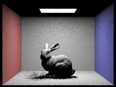
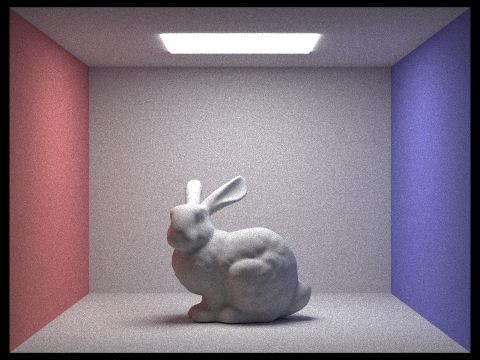
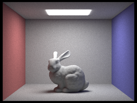
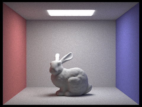
Hemisphere sampling contains a lot more noise than importance sampling. This is shown through the bunny that is smooth when we use importance sampling compared to the bunny with hemisphere sampling. Hemisphere sampling doesn't take into account all of the light that importance sampling does, which is why there's more noise in the hemisphere sampling because it doesn't have enough information.

Using importance sampling with a 1 sample per pixel rate leads to noise when we don't use enough light rays. Using a 1 sample per pixel rate doesn't get enough information to decrease the noise when we render. However, whenever we add more light rays the noise begins to decrease because there is more light hitting each pixel. Although the images are sharp, the more light rays do help with the noise.

Part 4: Global Illumination

For part 4.1, we implemented DiffuseBSDF::sample_f where we set pdf to 1/(2*pi) and wi to a randomly generated direction within our hemisphere and return f(wi->wo).

For part 4.2, we implemented indirect lighting with at_least_one_bounce_radiance by incorporating multiple bounces. We start off by returning an empty vector if our ray has a depth of 0. Otherwise, we keep a variable L representing our resulting radiance vector. We add the result of one_bonce_radiance to L and call sample_f on the bsdf of the intersected object in order to generate the reflectance (used for f_val), the pdf (used for p_val), and the randomly sampled direction within the hemisphere (used for w_i). We then create a Ray with the hit point as the origin and w_i converted to world space as the direction. We set min_t of this ray to EPS_F (for the same reasons as 3.3) and depth to the original ray subtracted by on (to be able to keep track of how many recursive calls were made and terminate appropriately). We then use this newly created ray to check if it intersects with any object in our BVH. If so, if it's the first time that at_least_one_bounce is being called and the max_ray_depth is greater than one (to satisfy the spec's requirement of having at least one indirect bounce) or if coin_flip of the continuation probability (we use 0.6) returns true, we add a recursive call to at_least_one_bounce_radiance on the new Ray and the new Intersection object, f_val, the dot product of the normal with w_i, all divided by p_val to L. The purpose of using coin_flip is to use Russian Roulette for an unbiased termination method.

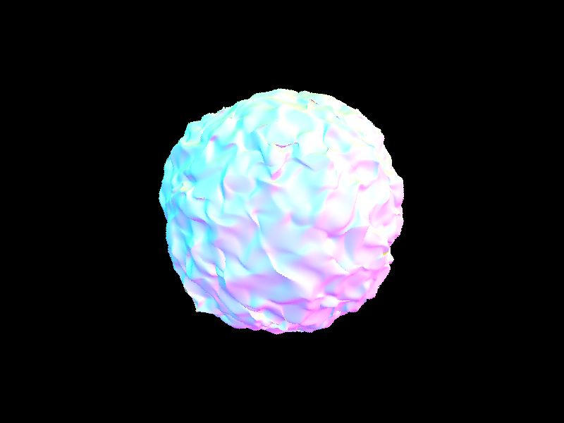
In part 4, we ran into many bugs. The main bug was that we were using importance sampling for one_bounce_radiance which caused shadows in the sphere we tried rendering to be much darker than they were supposed to be. We fixed this bug after several hours of looking through our at_least_one_bounce_radiance function, realizing that nothing looked wrong, and then checking other functions involved.

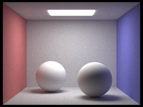
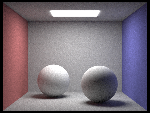
Direct illumination removes traces of noise unlike indirect lighting that does contain noise. There's nothing that removes the lighting in the direct illumination and it receives all the lighting. Shadows are harsher in the direct illumination unlike the indirect illumination that smooths out the shadows.

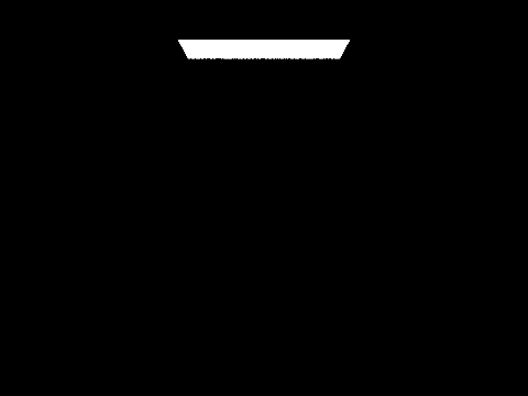
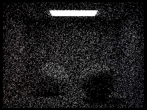
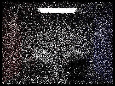
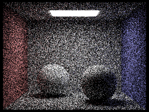
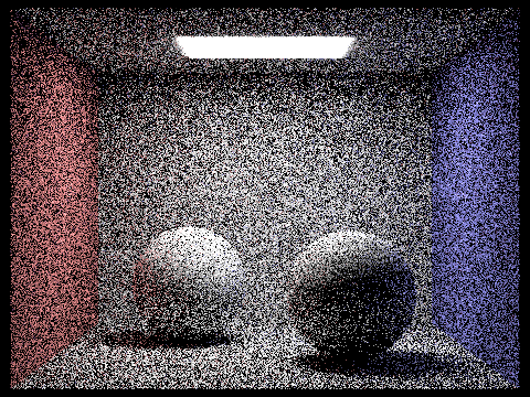
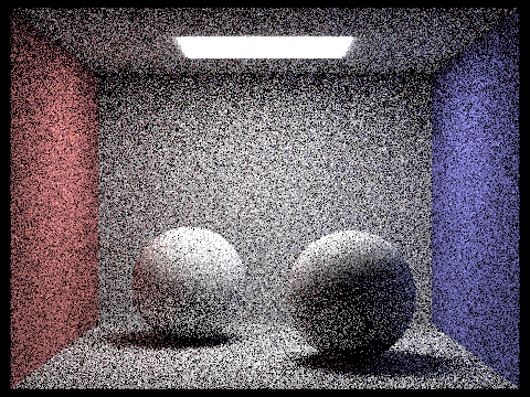
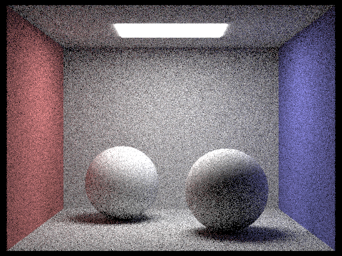
Changing max_ray_depth while using 1024 samples per pixel changes the image. Using a 0 max_ray_depth allows no light to come in except the light source which leads to a black room. Allowing 1 max_ray_depth we get direct illumination with harsh shadows and no noise. Increasing max_ray_depth after 1 starts to include noise and the image starts to get a little lighter and turns into indirect illumination.

Using 4 light rays with varying pixel rates results in a different image. With only 1 sample per pixel, the image looks graining and the colors are barely there. This is not enough samples to get the actual image. Slowly increasing the sample pixel rate increases the color and visibility of the image. The noise also decreases because we have more samples to get more information from. Using a higher sampling rate with only 4 light rays allows for a better image but not a perfect one.

Part 5: Adaptive Sampling

For part 5, we implemented adaptive sampling by updating our raytrace_pixel function to stop when sampling reaches a specified confidence interval. First, we added s1 (a double which keeps track of the summation of the illumination of each radiance sampled) and s2 (a double which keeps track of the summation of the illumination squared of each radiance sampled). We then have a condition that returns true only every samplesPerBatch samples. This allows us to save time by not checking every sample. If the condition is met, we calculate the mean using s1 divided by the number of samples sampled. We also calculate the standard deviation by finding the square root of the variance calculated using s1 and s2. We then calculate 1.96 times the standard deviation divided by the square root of the total number of samples sampled so far. We then check that this value is less than maxTolerance over the mean. If it is, we terminate the loop and return the ray divided by the total number of samples sampled.

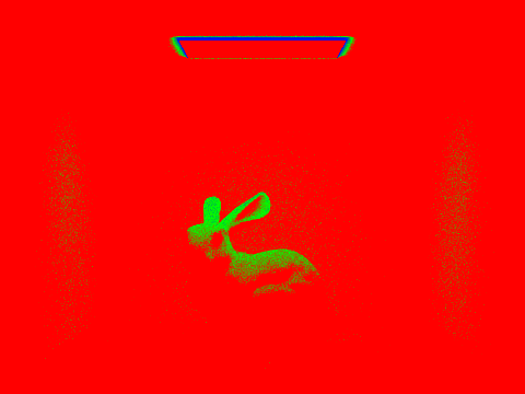
In the end, we failed to generate the image shown in the spec. Even though we went to four separate office hours to try to resolve the issue, we weren't able to fix it. We suspect an issue with our implementation for part 3 since for part 5, our values don't converge below maxTolerance as much as we need them to. Though this might be an issue with our part 5 calculations, we suspect instead that est_radiance_global_illumination is outputting a radiance that isn't bright enough, causing the values to not converge. We tried changing different variables to try to manipulate the radiance values to be higher, but to no avail. In the end, we hard-coded maxThreshold to be 0.2 in order to avoid rendering a completely red image.

Partner Reflection

For this project, we collaborated at the beginning of the project by both working on the same part and bounced ideas back and forth. We went to office hours and project parties to get the most work done while also getting help from TA's. We would split work but communicated to update each other and stay on track to finish the project. We learned a lot about the rendering process and how lighting affects images.

Link to repo: cal-cs184-student.github.io/sp22-project-webpages-maleny25/proj3-1/index.html