Link to (this) Webpage

Link to Code

Overview

In this project, we implement real-time simulation of cloth using a system based on masses and springs. We build the data structures to contain point masses and springs for our cloth, and we defined physical constraints to them. We used Verlet numerical integration over time to simulate the cloth movement. We also implemented constraints to avoid collisions with other objects as well as self-collisions accelerated with a spatial hash map. Finally, we implemented various shaders for our cloth and environment, including Diffuse, Blinn-Phong, Texture Mapping, Bump & Displacement Map, and Mirror.

As extra credit, we implemented a custom shader and also simulated wind!

Part 1: Masses and springs

Here we have our cloth wireframe showing the structure of our point masses (vertices) and springs (edges):

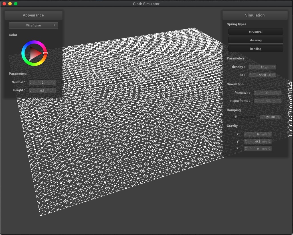
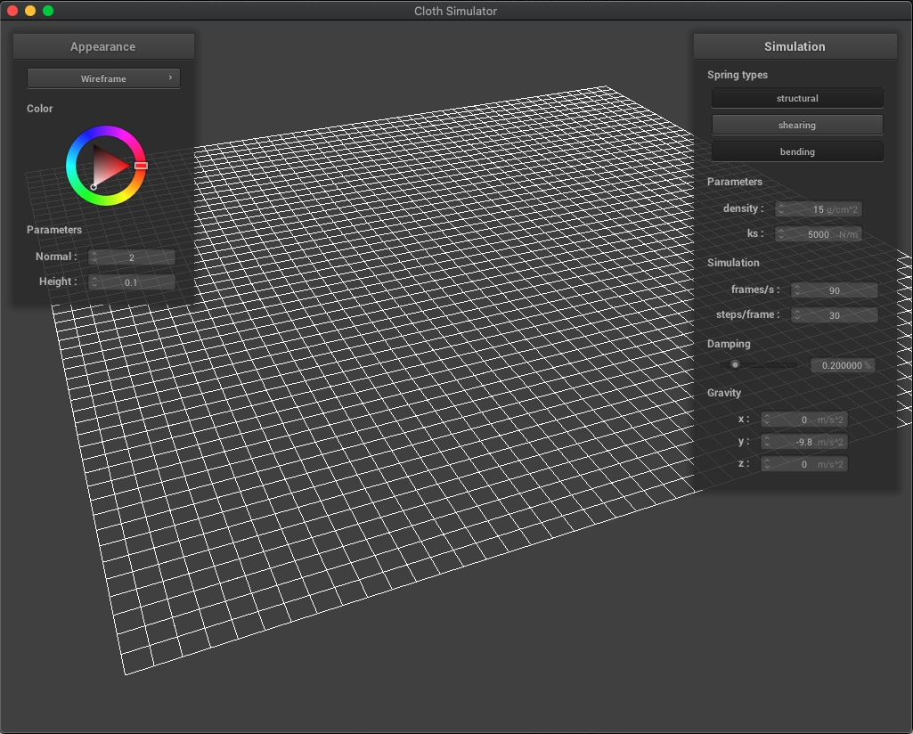
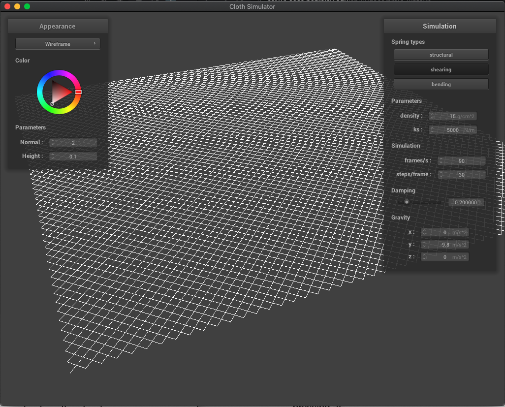
We also present our wireframe without shearing constraints (where we only see horizontal and vertical springs), only shearing constraints (diagonal springs), and with all constraints:

(1) No shearing	(2) Only Shearing
(3) All constraints

Part 2: Simulation via numerical integration

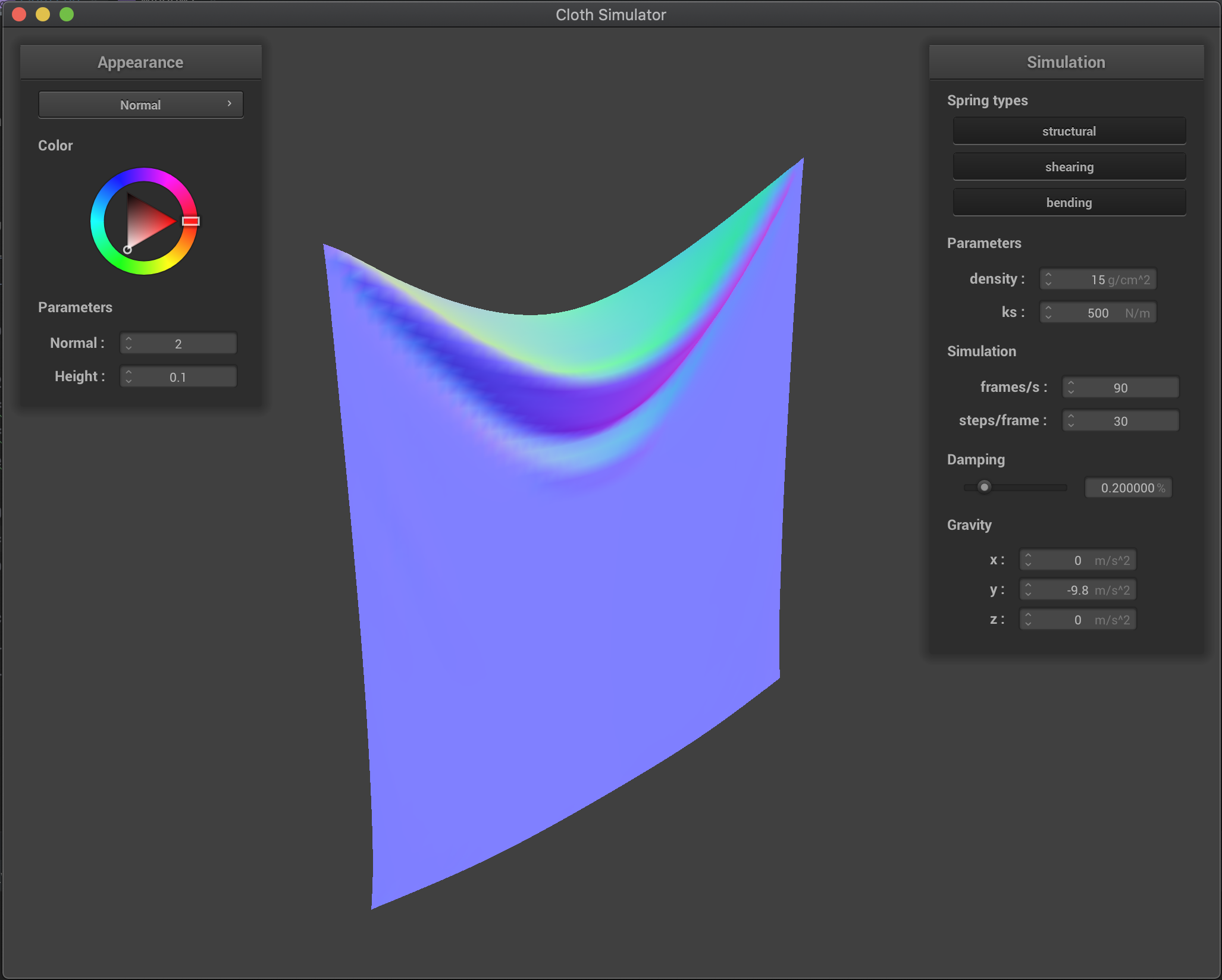
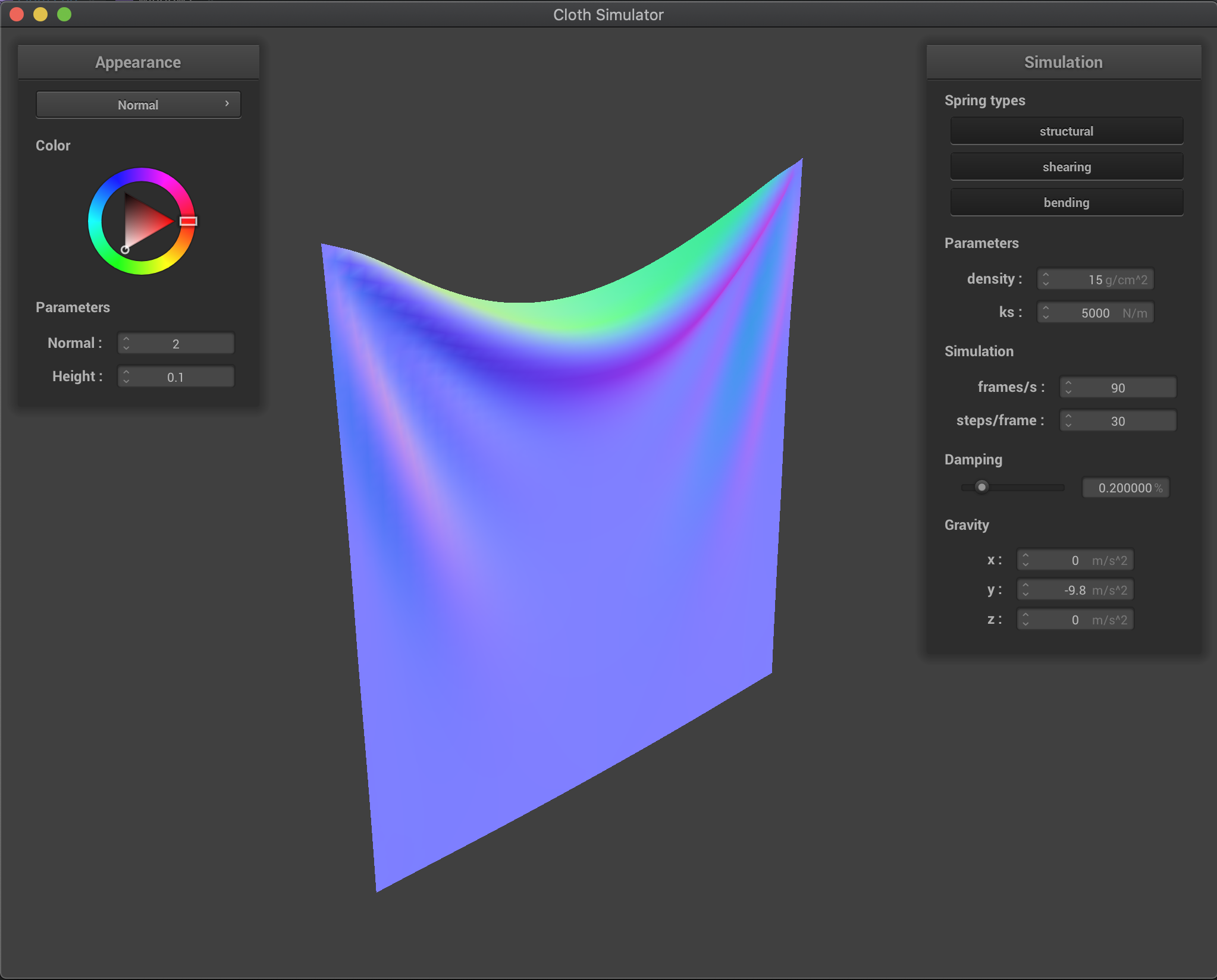
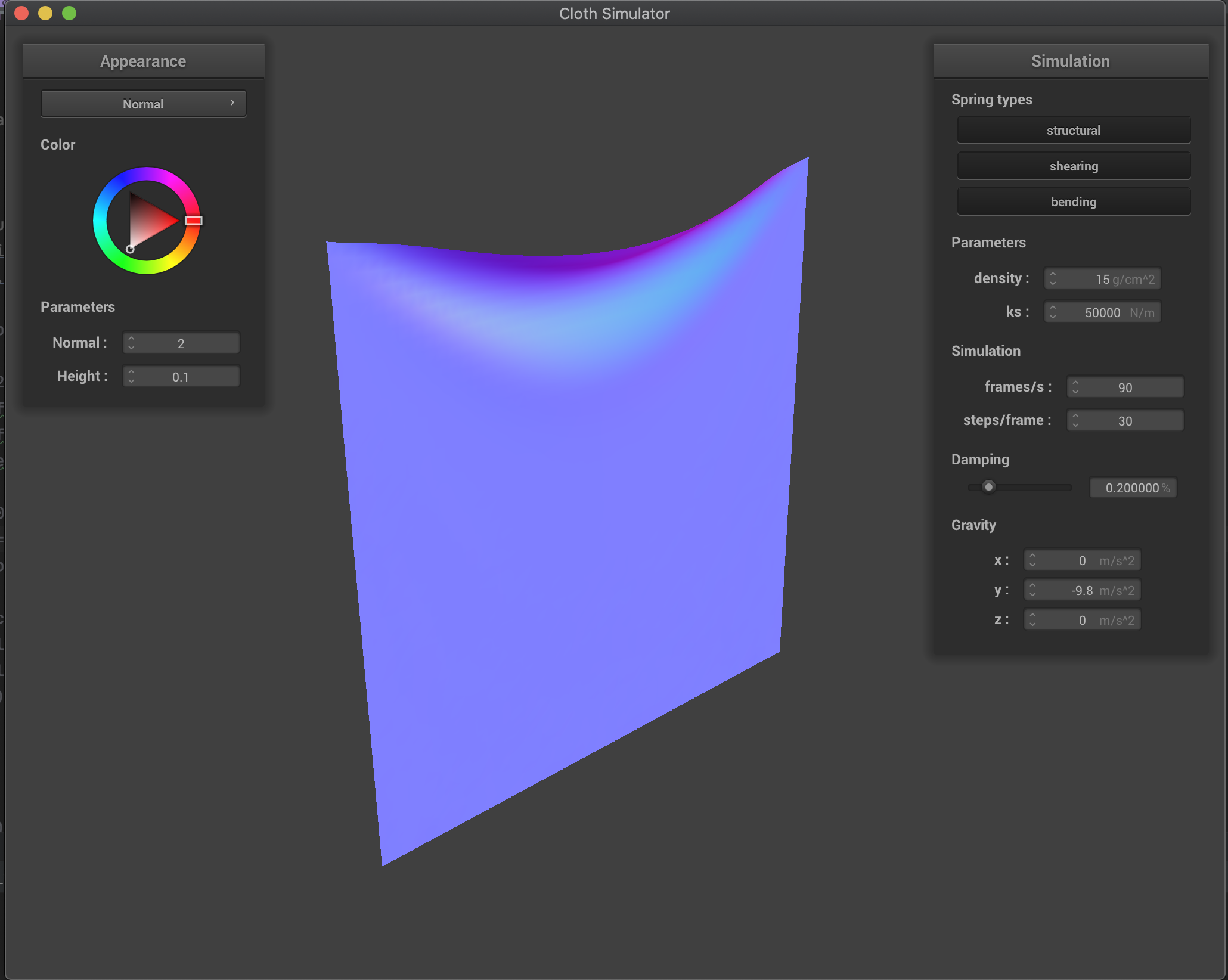
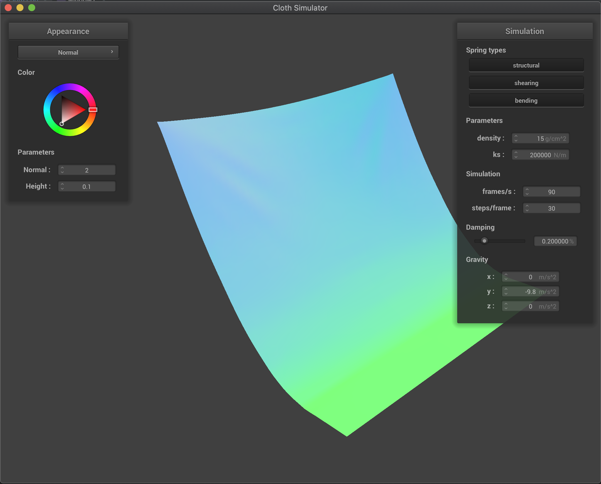
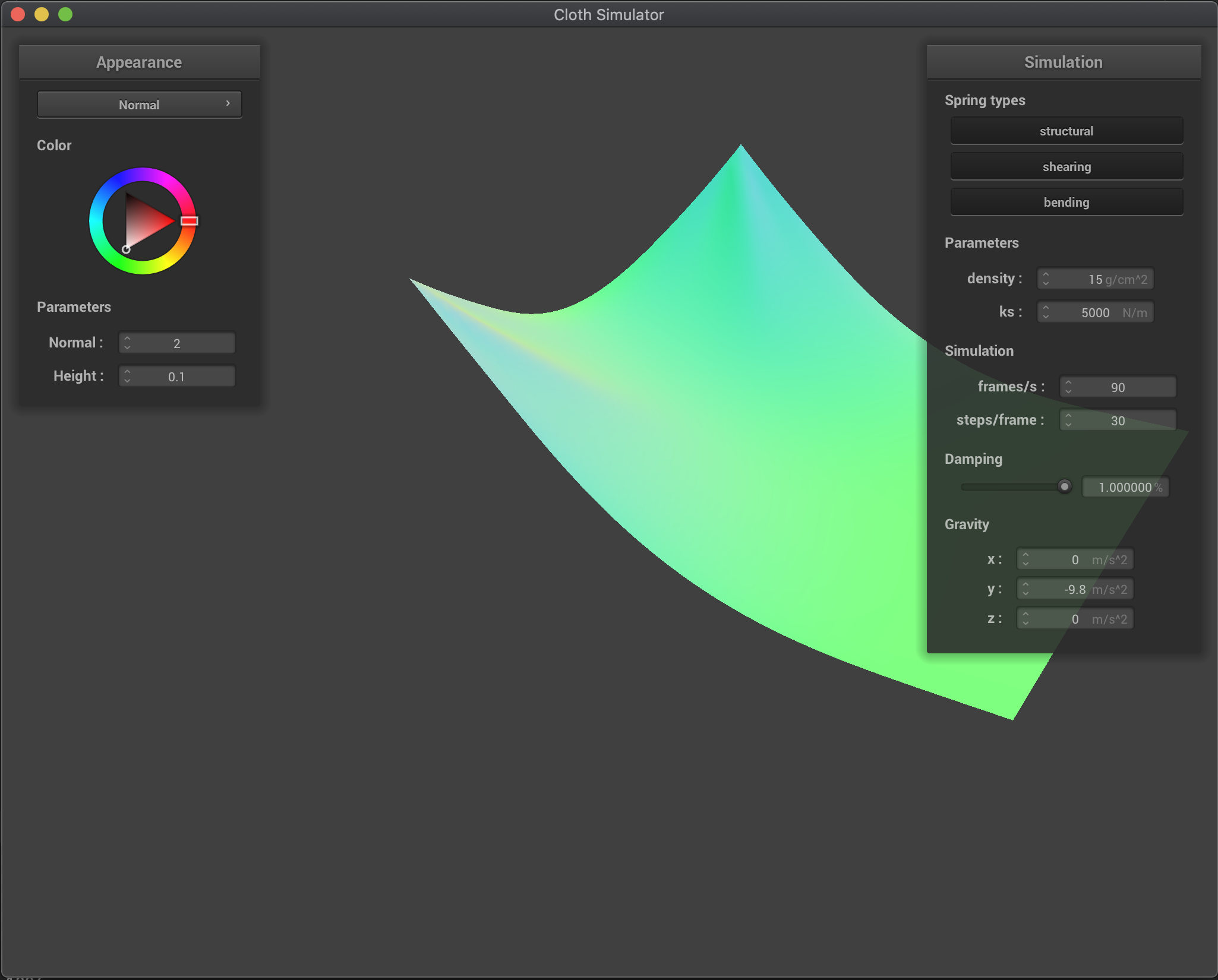
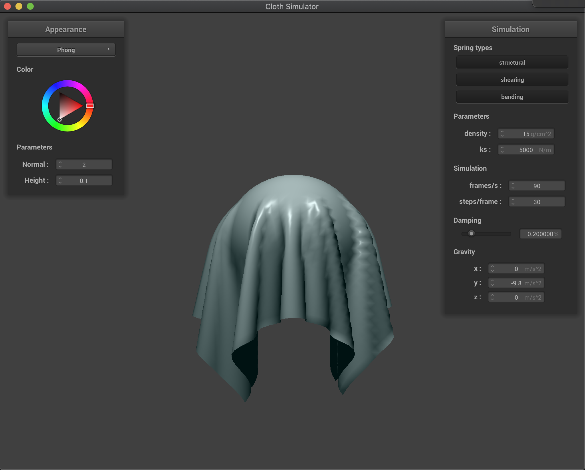
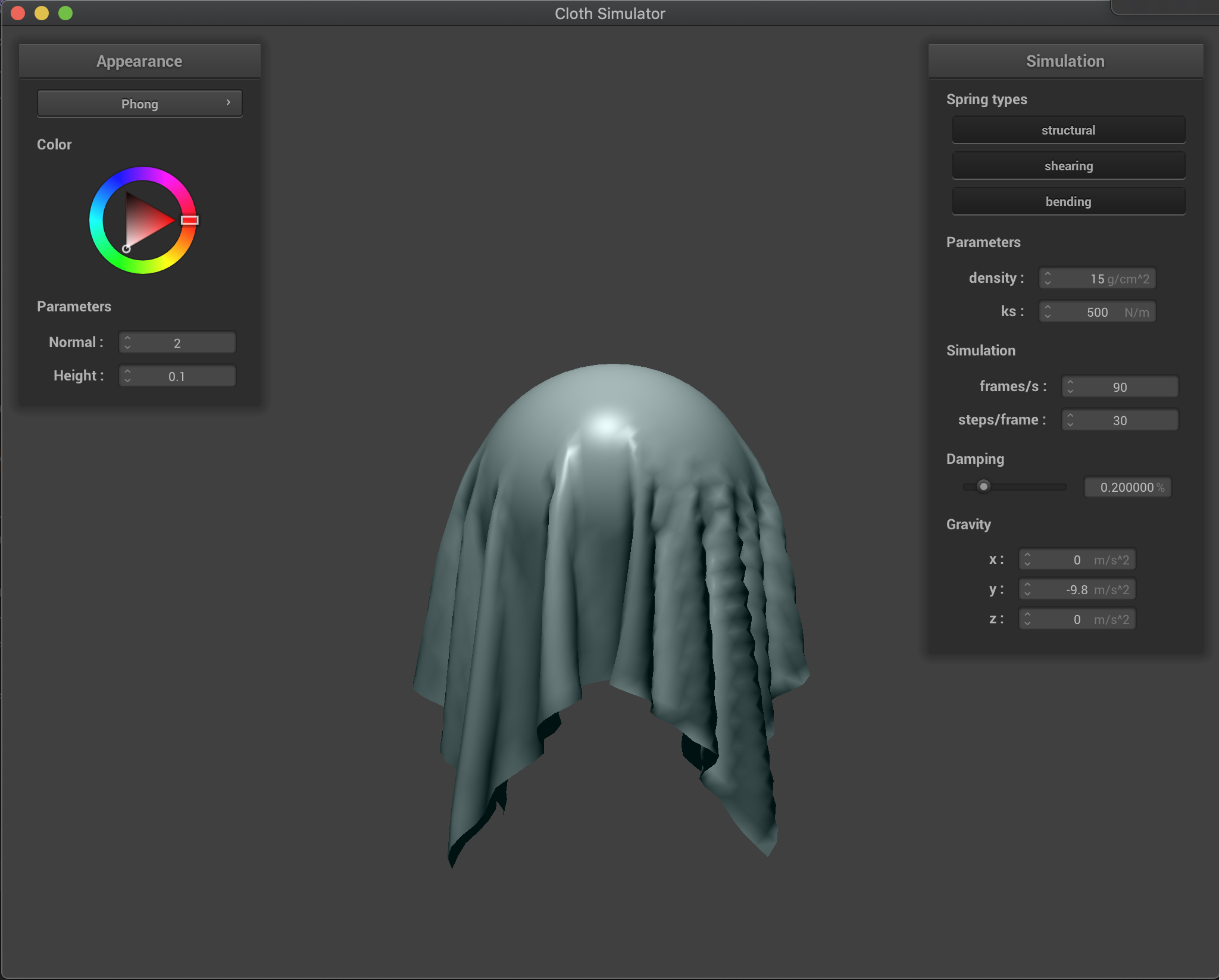
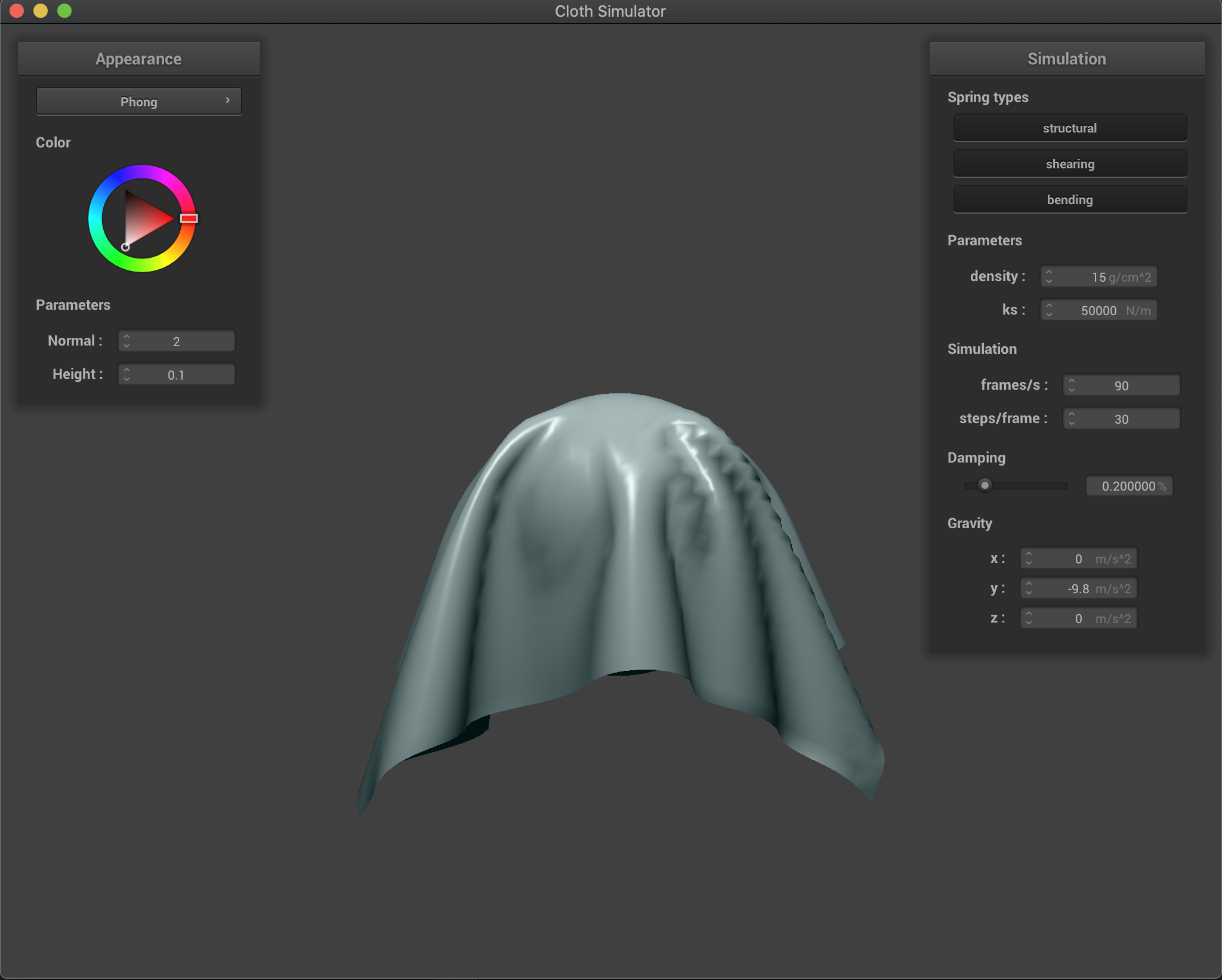
Effects of spring constant ks

We have that with a larger ks the cloth is more rigid and less flexible. On the other hand, a smaller ks allows for a more flexible and elastic cloth. However, for a very small ks, we have that mostly the cloth behavior is dominated by the 10% elongation constrain since here the spring forces alone are not enough to hold the cloth against gravity.

Here we show the intermediate or resulting state for various values of ks:

ks = 500	ks = 5000 (default)
ks = 50000	ks = 2000000

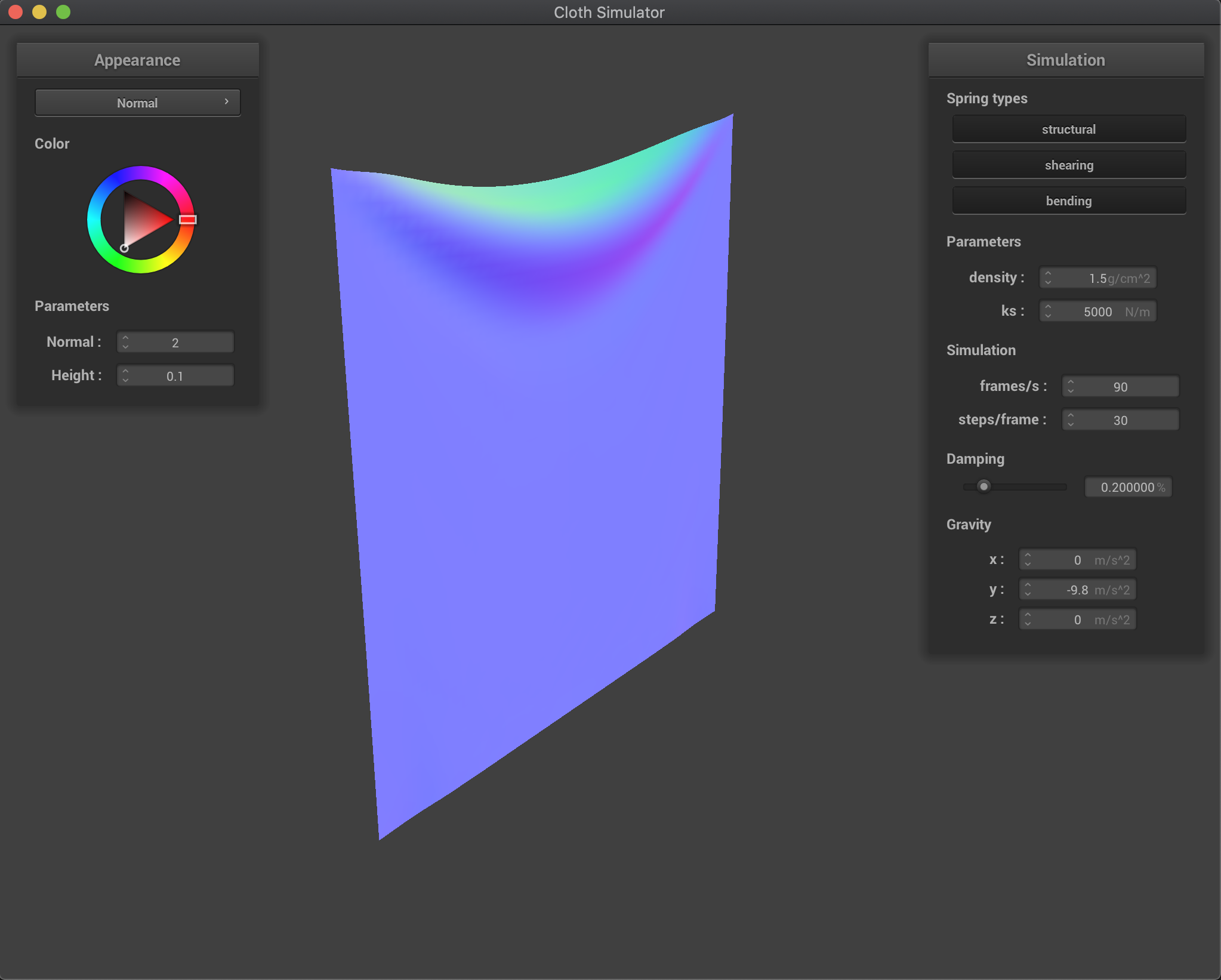
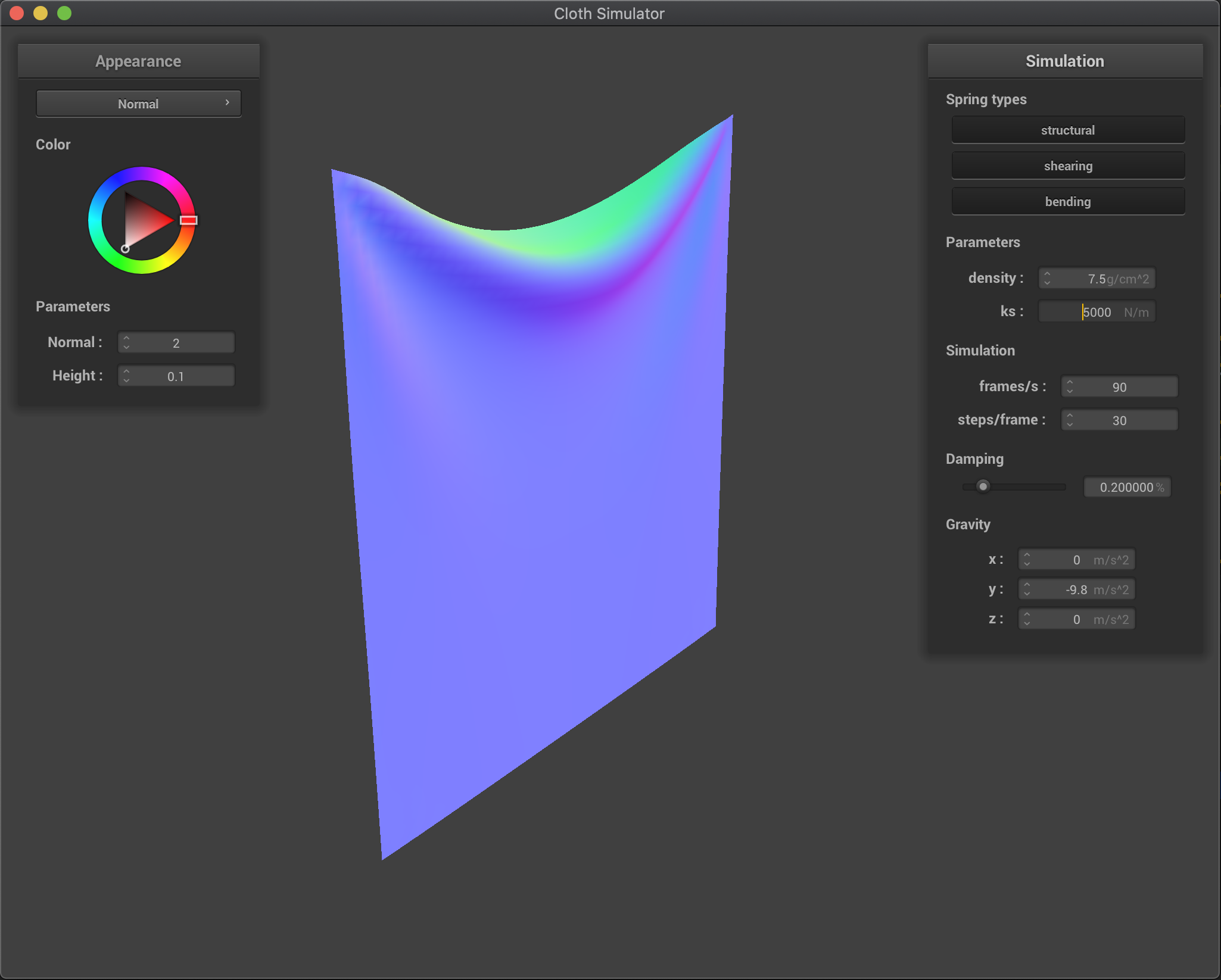
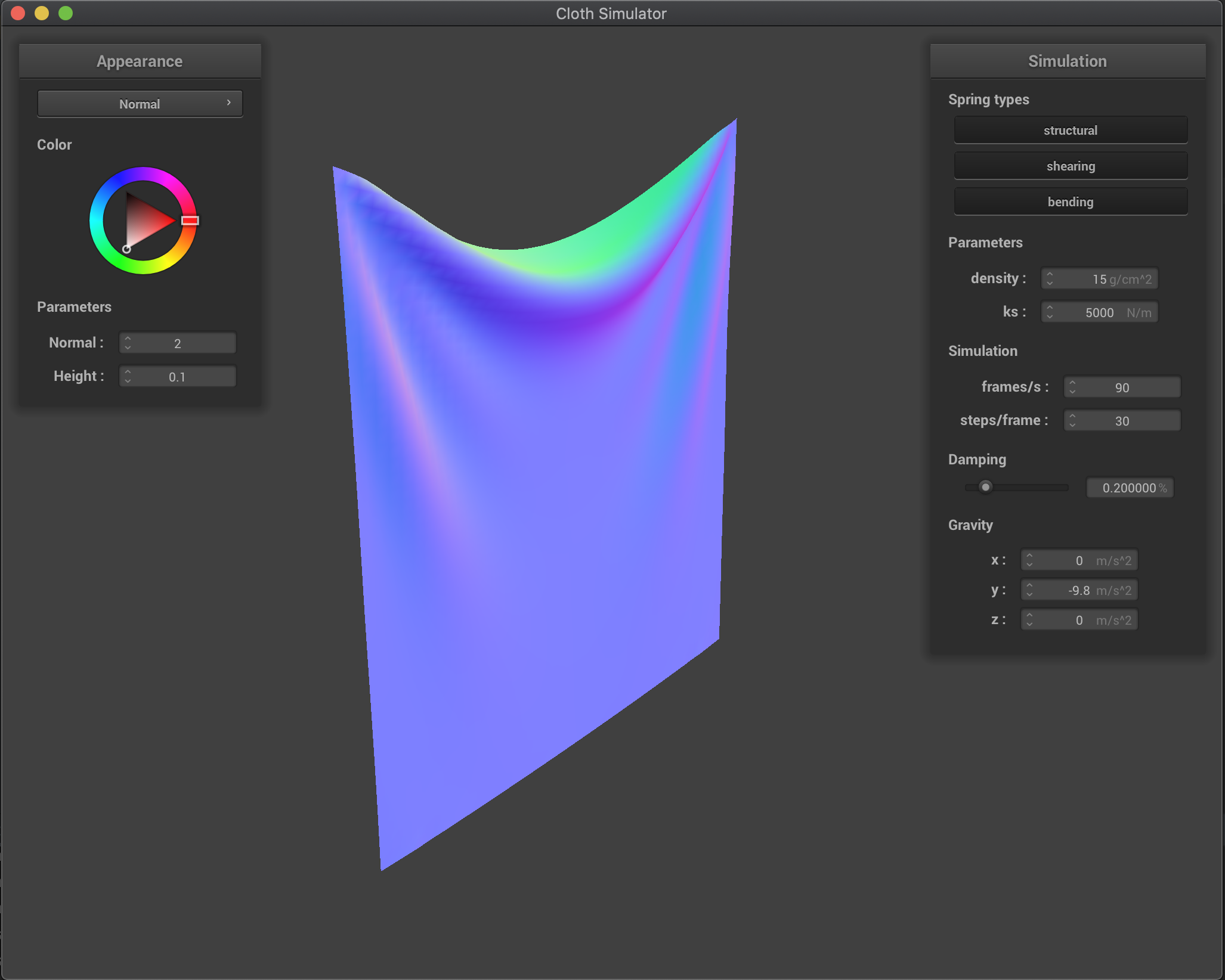
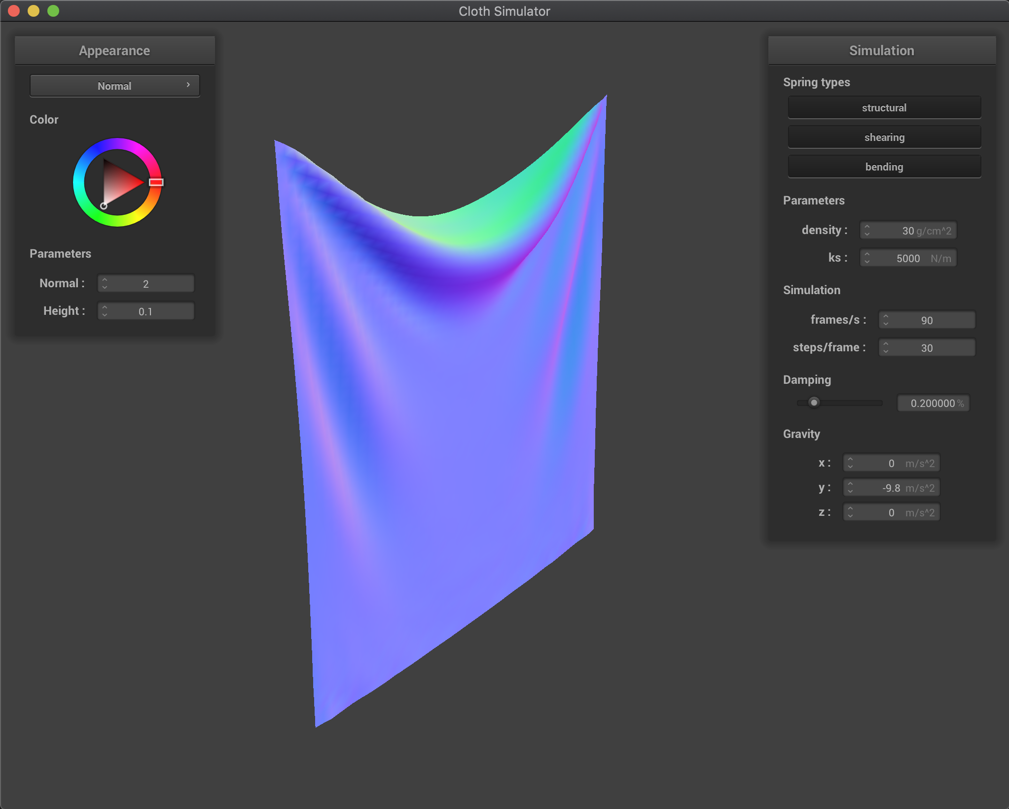
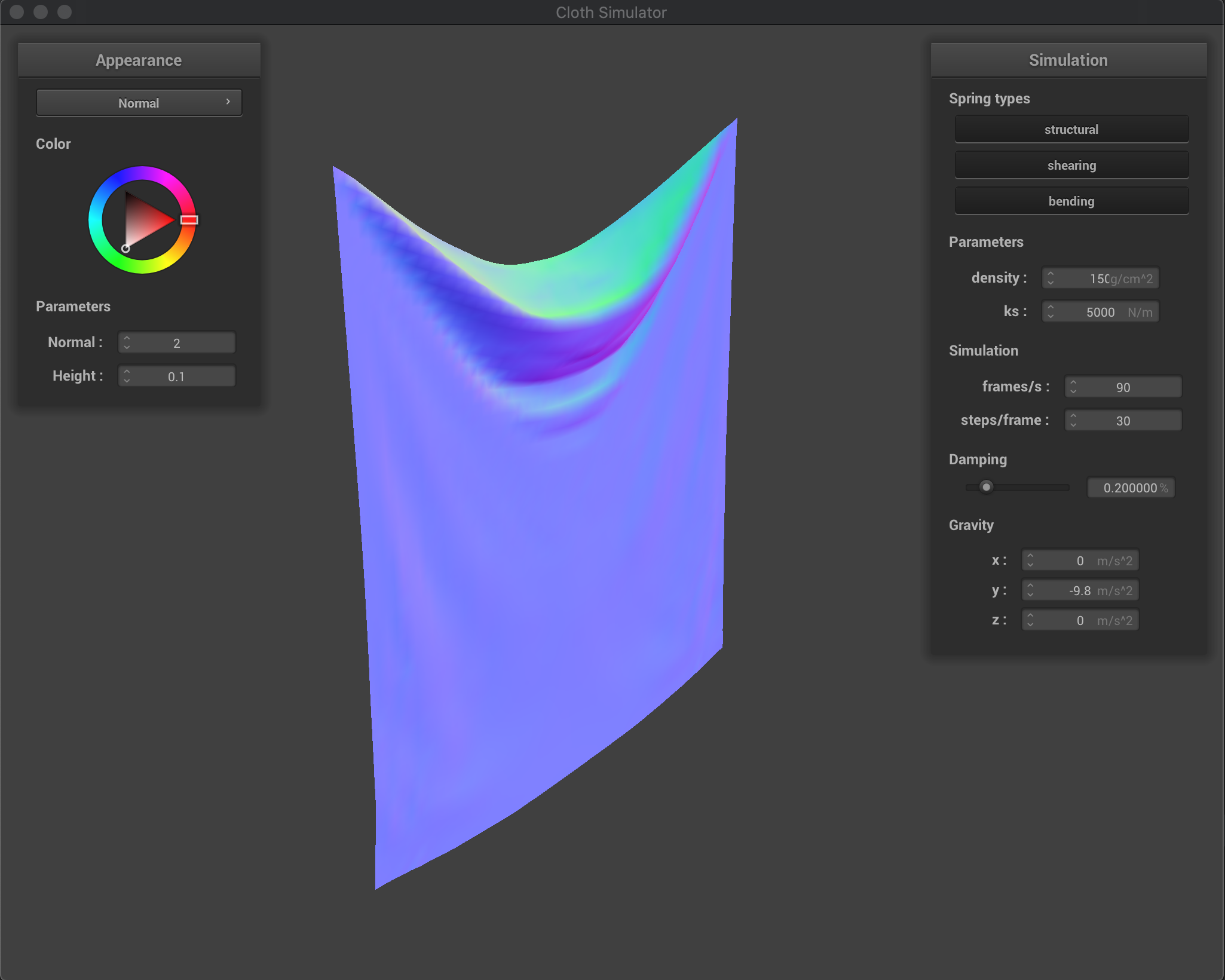
Effects of density (in g/cm^2)

Increasing the density produces a more heavier cloth, which Effects of varying the density are similar to the inverse of the effects from varying ks. We have that by decreasing the cloth density, external forces (gravity) are reduced while the spring forces remain the same (another way to analyze is that since now the mass is lower, the acceleration produced by springs is larger - keeping gravity acceleration the same). Therefore, we have that the ratio of gravity force vs spring forces increases as we increase the density. This produces a heavier cloth that will deform more as we increase density, as it can be seen in the figure below.

density = 1.5	density = 7.5
density = 15 (default)	density = 30
density = 150

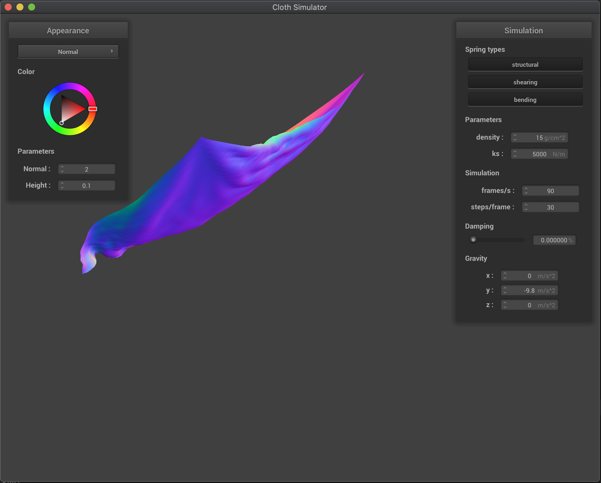
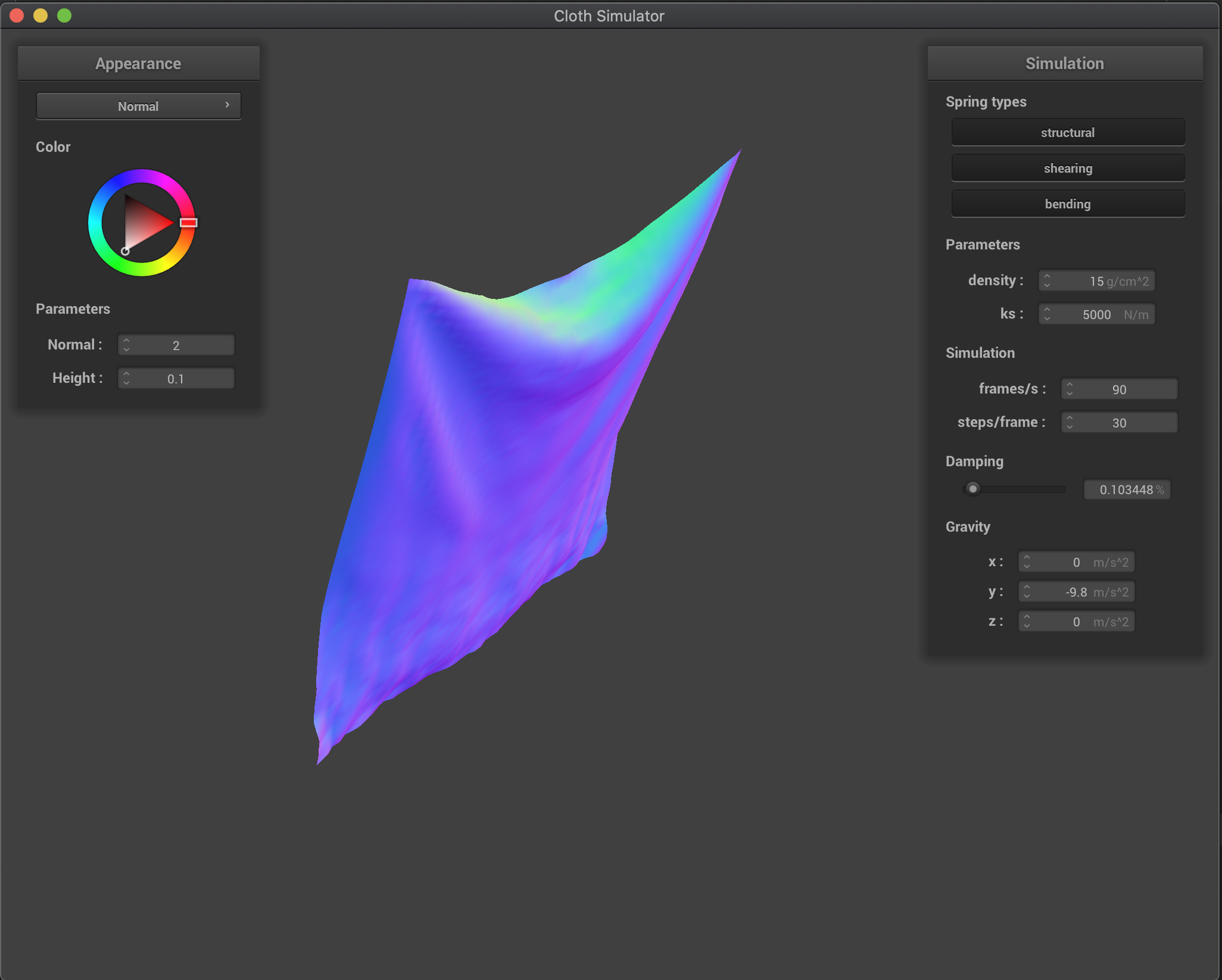
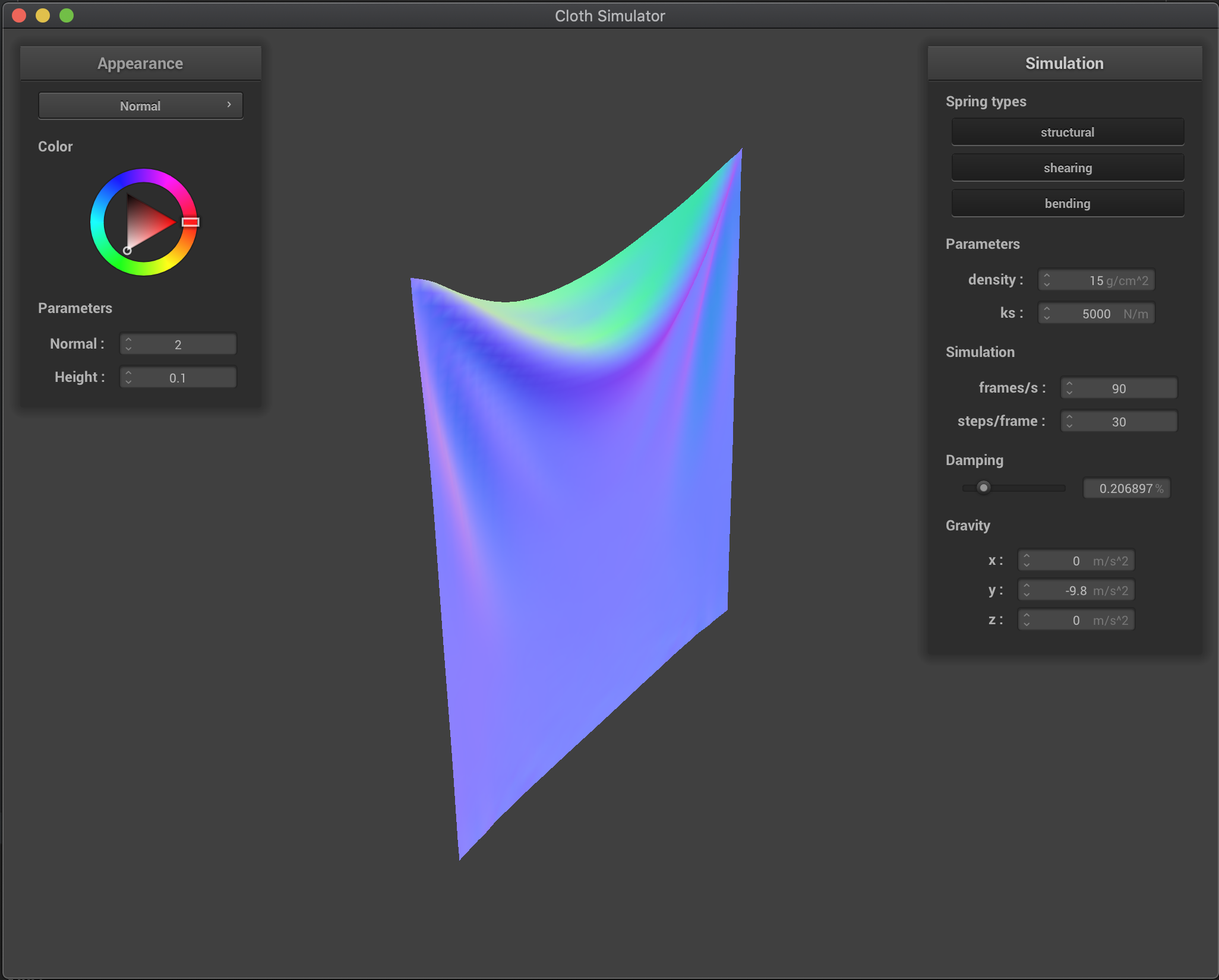
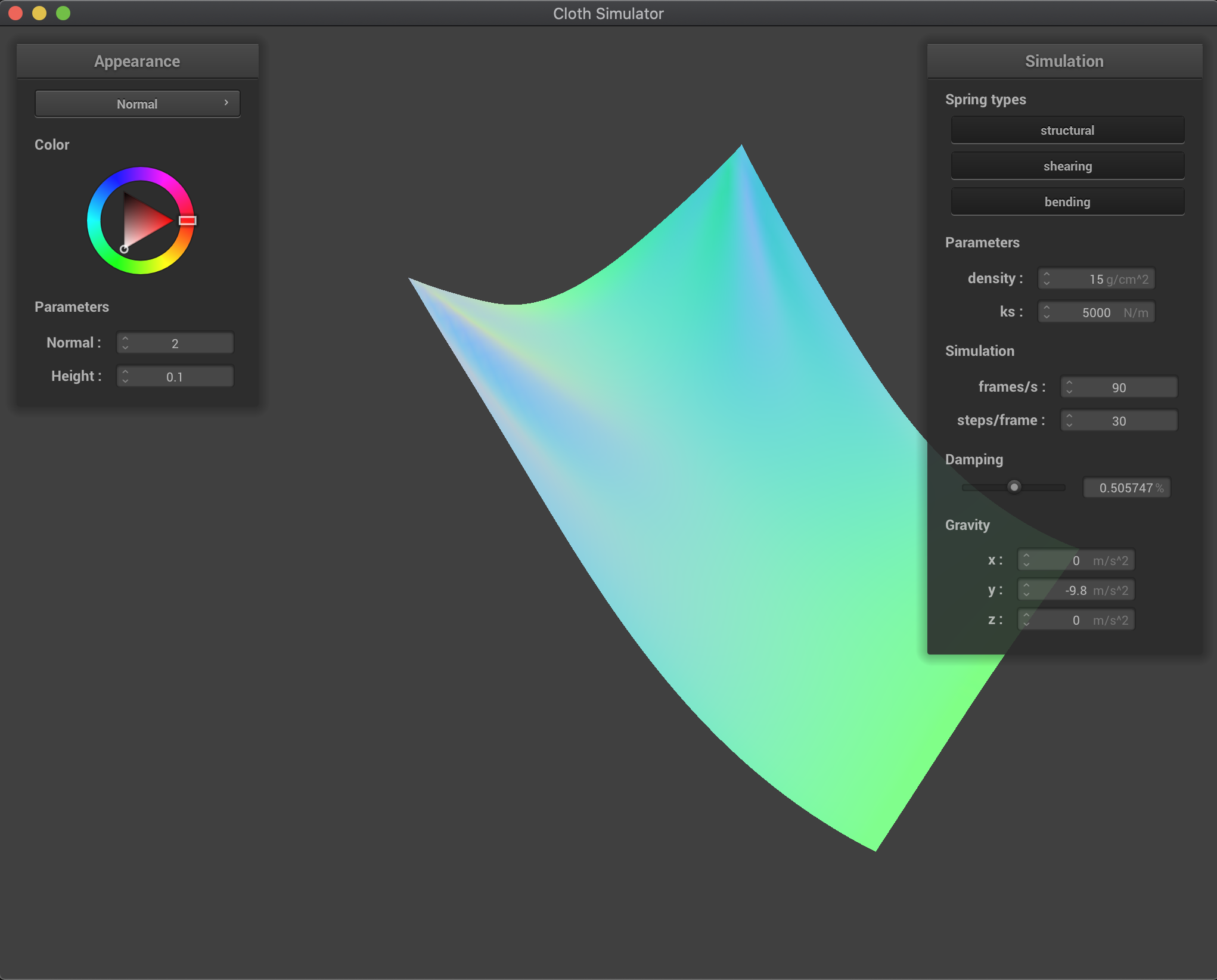
Effects of damping

Increasing the damping percentage parameter makes our cloth fall more slowly and makes it look more rigid. Basically, by increasing the parameter, we are losing more energy (velocity in our case) while we fall and we smoothly converge to the final rest state. On the other hand, when we decrease damping, the cloth fall is much quicker and the cloth deforms much more, and we start to overshoot the final rest state and oscillate before converging. In the extreme case of no damping (damping=0), the cloth overshoots the convergence state and goes back up a lot and oscillates for a long long time (I didn’t wait to see if it would eventually converged since it was taking quite a bit of time). This makes sense: if there’s no energy losses, there’s no reason for the cloth to reach a lower energy state (lower height and zero speed), so it makes sense for the cloth to keep going. However, even though there’s no damping in this last case, there is some “energy losses” due to our model approximation: for example, we limit the maximum extension of our springs to 10% over their rest length, altering the natural behavior of the point masses and not respecting energy conservation laws.

damping = 0.0%	damping = 0.1%
damping = 0.2% (default)	damping = 0.5%
damping = 1.0%

Final resting state for default parameters

The final state for the default parameters produces a nice and realistic resting state for the cloth, where we have some folding in the middle where most of the cloth weight has to be supported, and smoothly flattens as we go lower:

Part 3: Handling collisions with other objects

Sphere

Below we show the final resting state for our cloth collision with the sphere for multiple values of our ks parameter. As described in the previous section, a smaller ks decreases our spring forces and makes our cloth more flexible and stretchy, as it can be seen in the figure below for ks=500 where the cloth stretches more and reaches lower positions. On the other hand, a larger ks parameter increases our cloth spring forces obtaining a more rigid cloth. This can be seen in the figure below for ks=50000 where the cloth tries to stay more flat and stretches much less. We took the freedom to use the Blinn-Phong shader for more beautiful results.

ks = 5000 (default)	ks = 500
ks = 50000

Plane

We can see that collisions with the plane work as well! The cloth nicely rests on the plane without going through (we show a view from above the plane and another from below the plane). We used the texture shader for a nice contrast between cloth and plane!

View from above plane	View from below plane (cloth does not go through)

Part 4: Handling self-collisions

With self-collision, we can see the cloth folding on itself rather than clipping through it.

Early, initial self-collision	Intermediate state
Restful state	Entire Simulation (GIF)

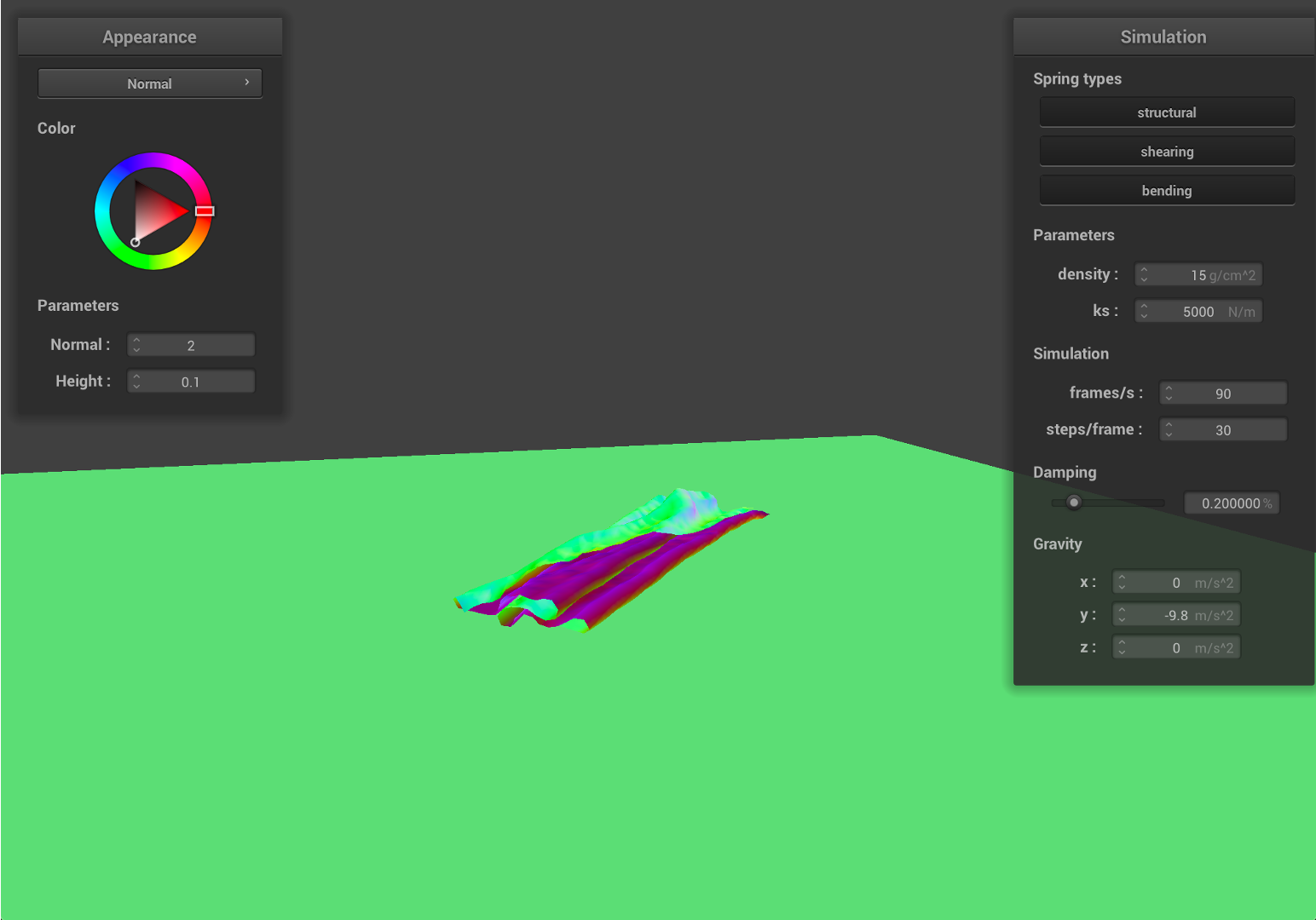
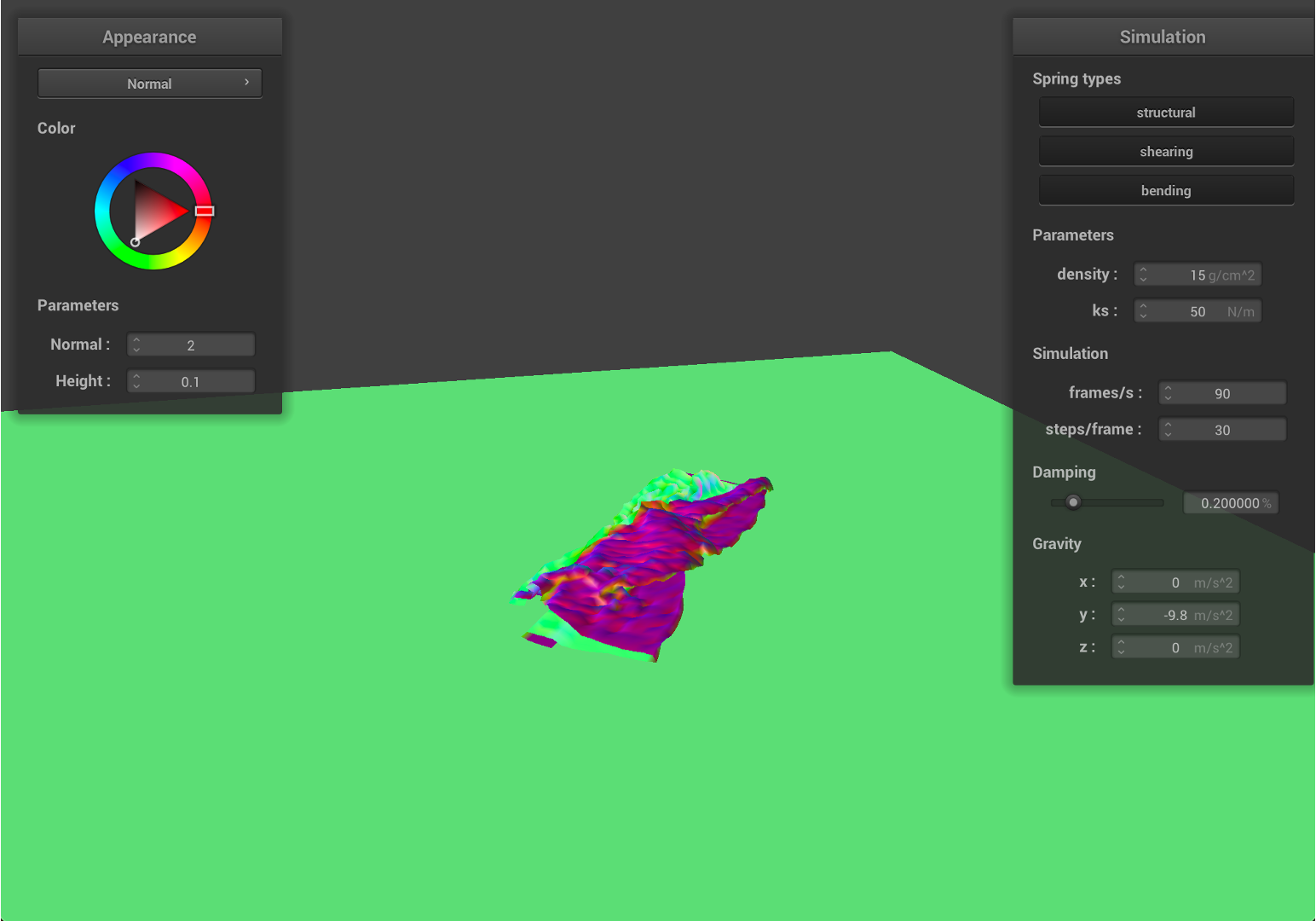
How different density and ks affect the behavior

• First, we decrease the density to 1, which indicates that the material become 15 times lighter.

Early, initial self-collision	Intermediate state
Restful state	Entire Simulation (GIF)

As we can see from the results, the falling cloth has much less folding and smother surfaces. Since the mass is much smaller, given the same ks, the local deformation become smaller, therefore, the cloth will have less stretching and results in a smother surface.

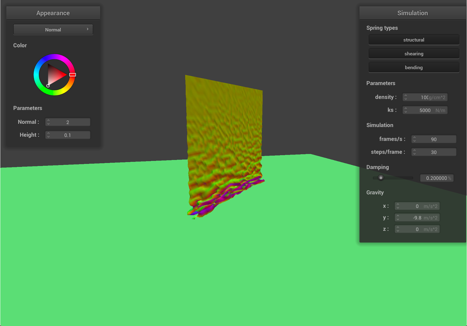
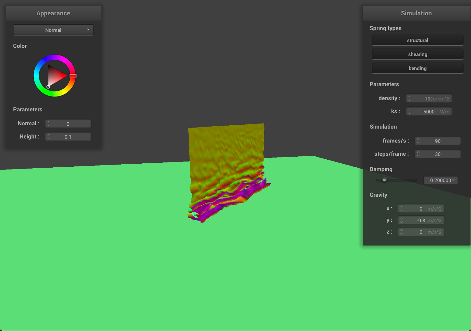
• Now, we increase the density to 100, which indicates that the material become around 7 times denser or heavier.

Early, initial self-collision	Intermediate state
Restful state	Entire Simulation (GIF)

As we can see from the results, the falling cloth has much more folding and rougher surfaces. Since the cloth is much heavier, given the same ks, the local deformation become bigger, therefore, the cloth will have much more stretching and results in a rougher surface. Due to the deformation, the cloth will have smaller surface area compared to the initial state.

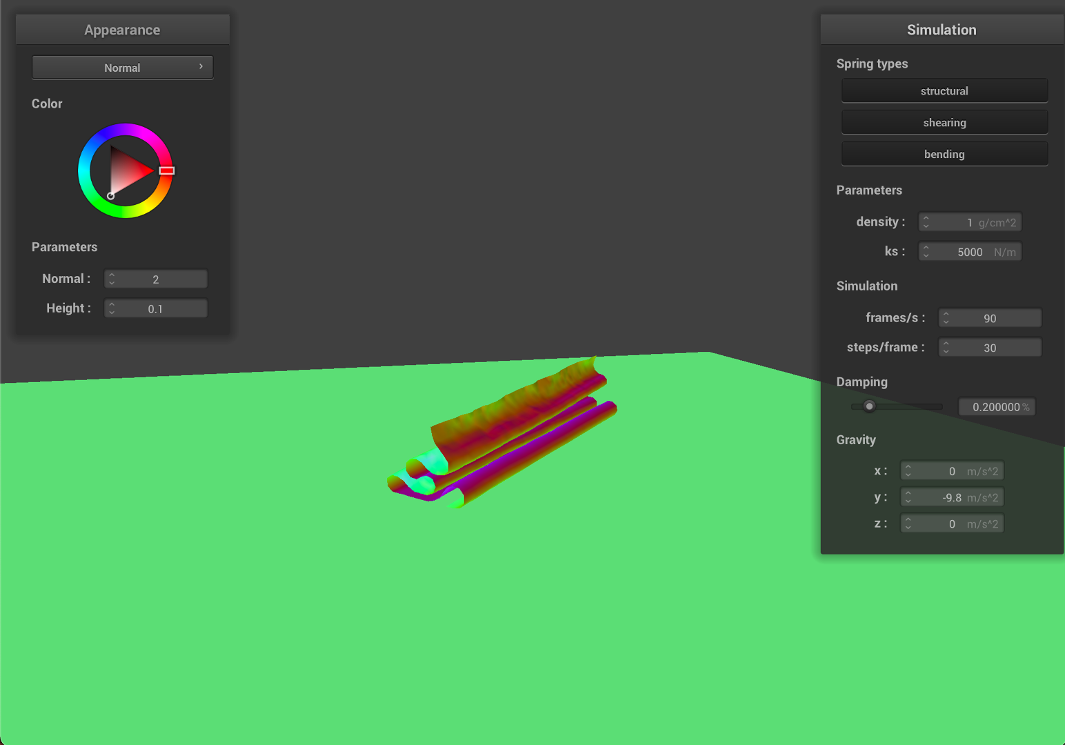
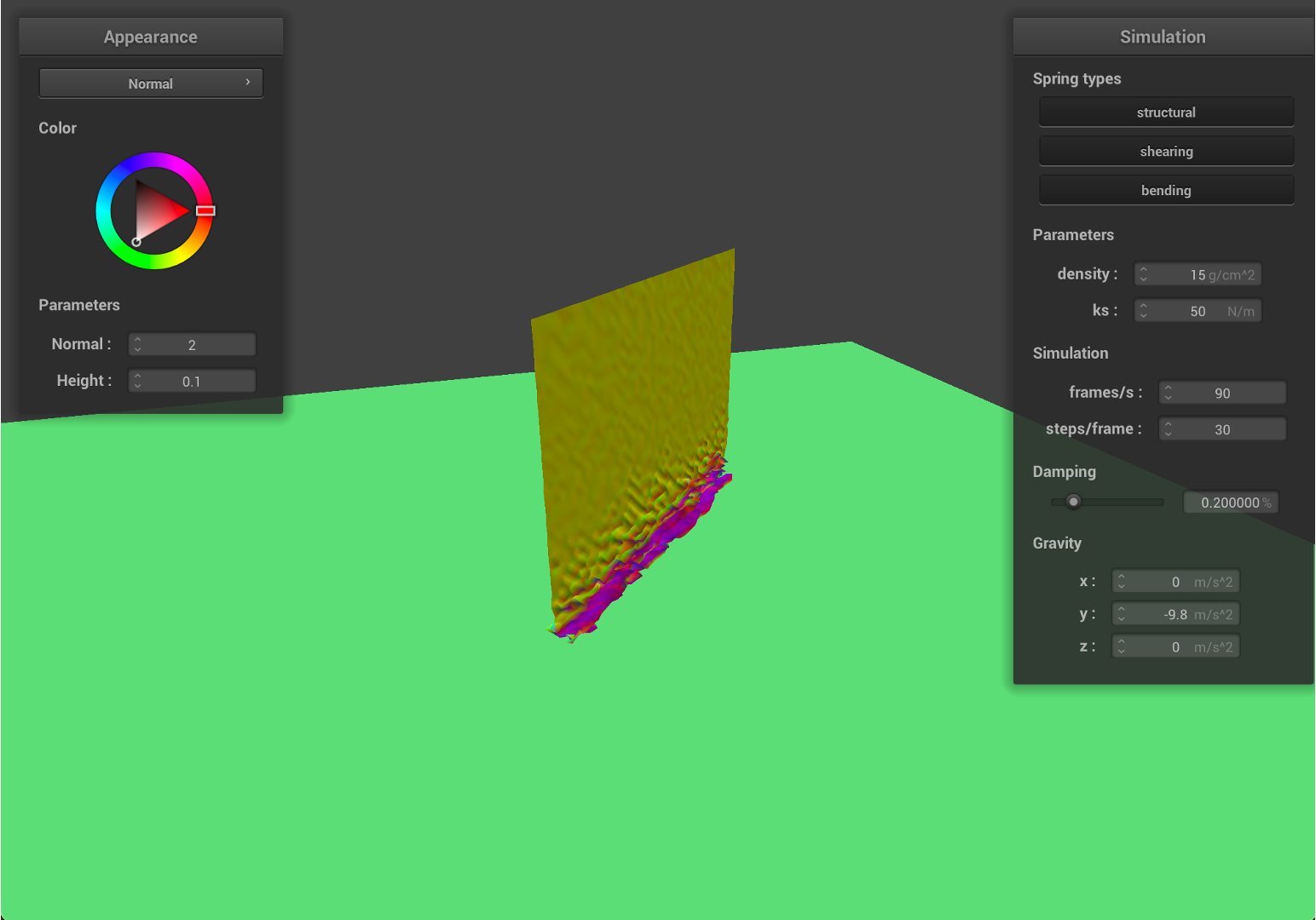
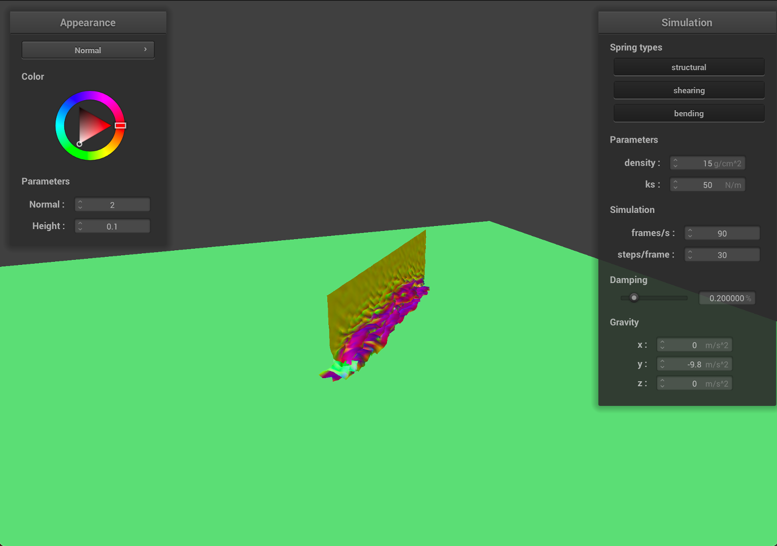
• Now, we decrease ks to 50, and set the density as 15, with smaller ks, the springs will have larger deformations with the same force on it.

Early, initial self-collision	Intermediate state
Restful state	Entire Simulation (GIF)

As we can see from the results, the falling cloth has much more folding and rougher surfaces, which is similar to the effect with higher density value. Since ks is smaller, given the same density value, the local deformation become bigger, therefore, the cloth will have much more stretching and results in a rougher surface. Due to the deformation, the cloth will have smaller surface area compared to the initial state.

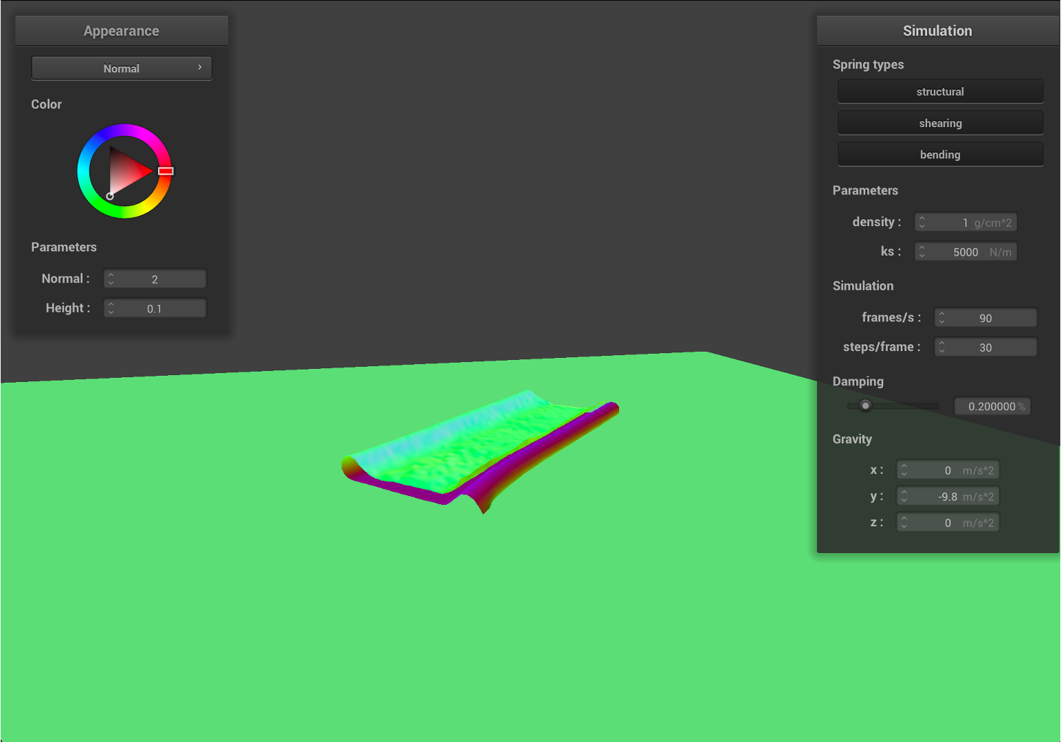
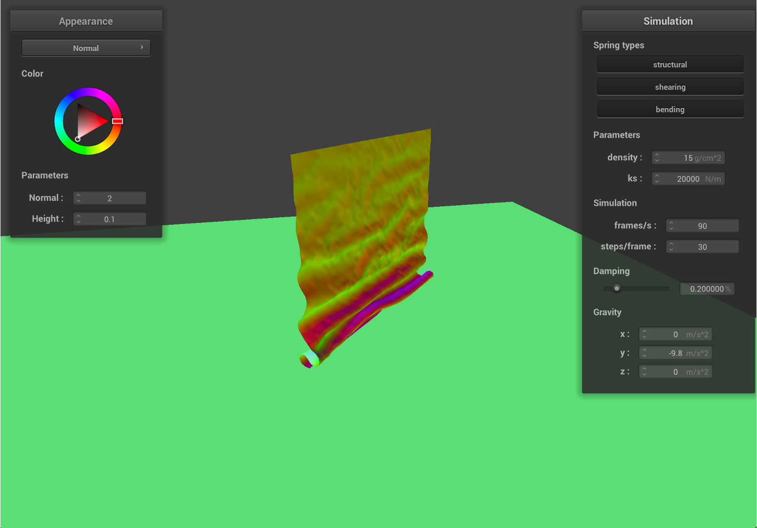
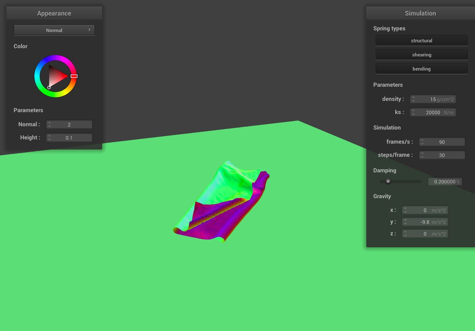
• Now, we increase ks to 20000, and set the density as 15, with larger ks, the springs will have less deformations with the same force on it.

Early, initial self-collision	Intermediate state
Restful state	Entire Simulation (GIF)

As we can see from the results, the falling cloth has much less folding and smother surfaces. Since ks has a much higher value, given the same density, the local deformation become smaller, therefore, the cloth will have less stretching and results in a smother surface.

Part 5: Shaders

1. Shader program:

Shader program (GLSL shader program) is a part of the graphic and rendering pipelines, which runs in parallel on GPU to accelerate the rendering process. Shader programs are used to create different lighting and material effect and properties (e.g., diffuse, mirror). In this project, we are primarily working on two shader types: vertex shaders and fragment shaders. Vertex shader manipulates each vertex of the rendered model and outputs the properties of the mesh (e.g.,normals, positions). We modified it to create the bumpy effects. The fragment shader determines the color of each pixel that is going to be rendered. In our experiments, the vertex shader outputs the mesh information that is further used in the fragment shader.

2. Blinn-Phong shading model

Blinn-Phong shading model accounts for three different lighting effects: 1) ambient lighting; 2) diffuse shading; and 3) specular reflection. Ambient lighting gives a uniform color without considering the lighting and the object geometry. Diffuse shading gives isotropic reflection. Finally, specular reflection determines more realistic reflections based on the material properties.

Cloth with ambient lighting	Cloth with diffuse shading
Cloth with specular reflection	Cloth with entire Blinn-Phong modeling

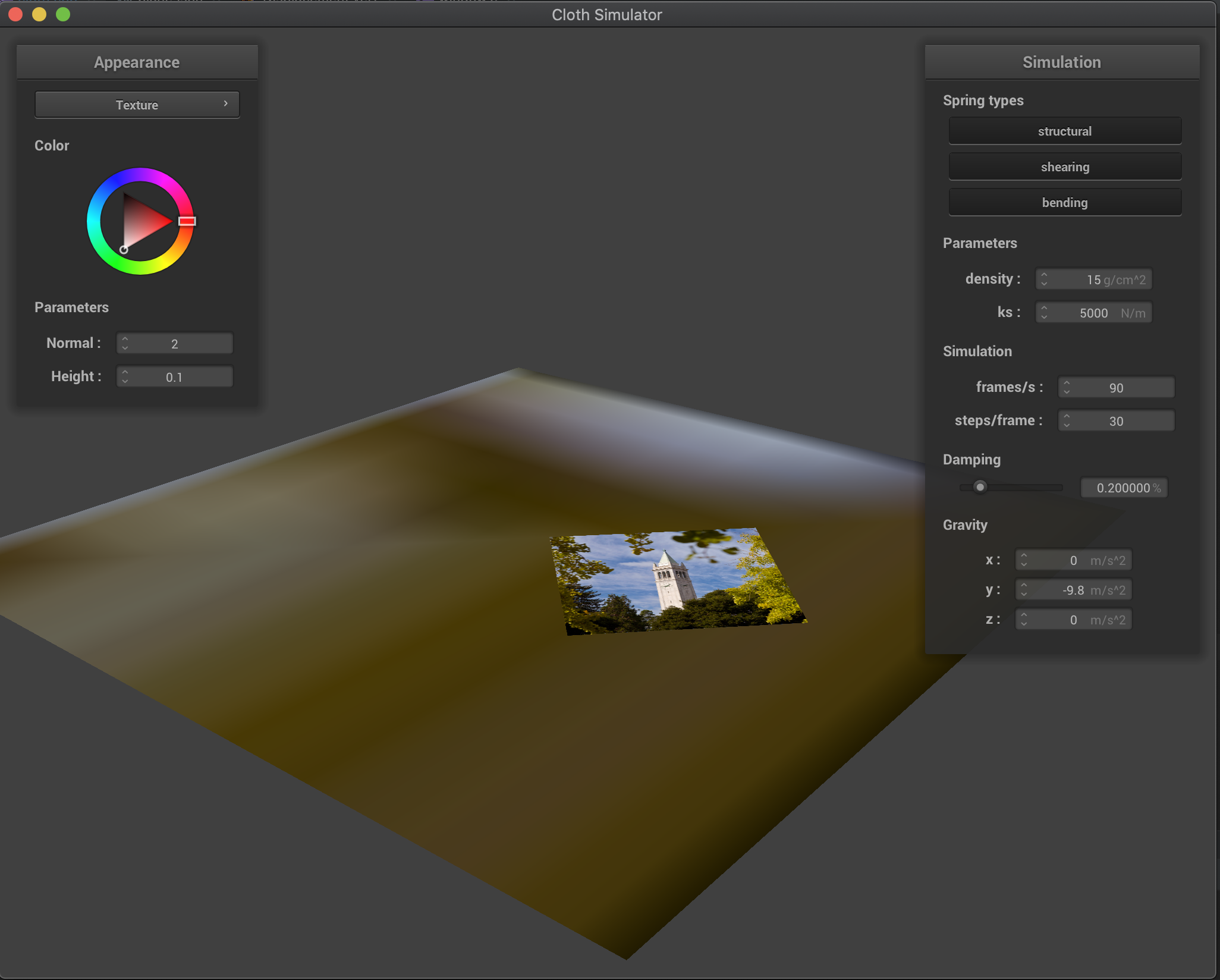
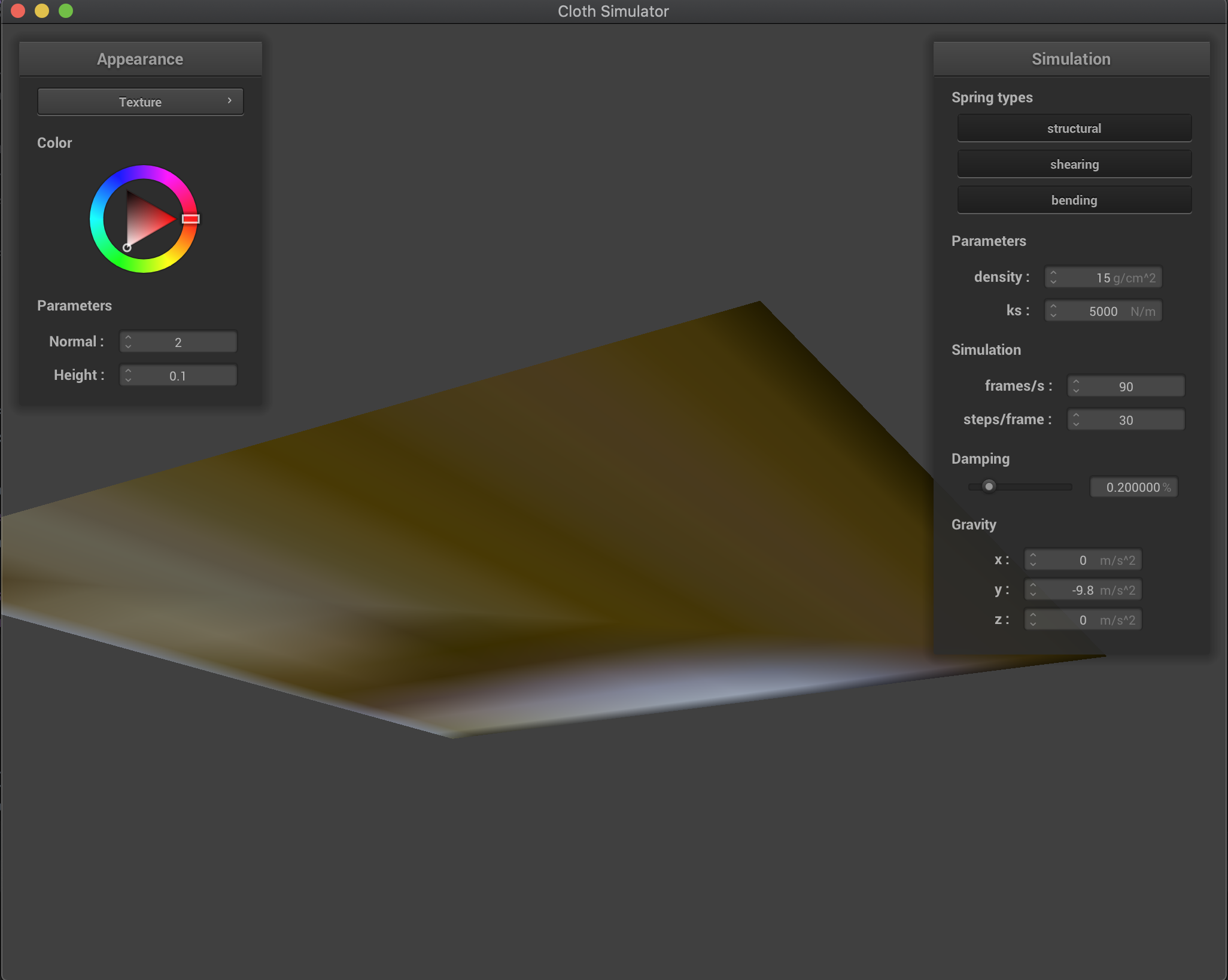
3. Texture mapping

We modified the textures to a cute cat - june, and show the simulation gif here.

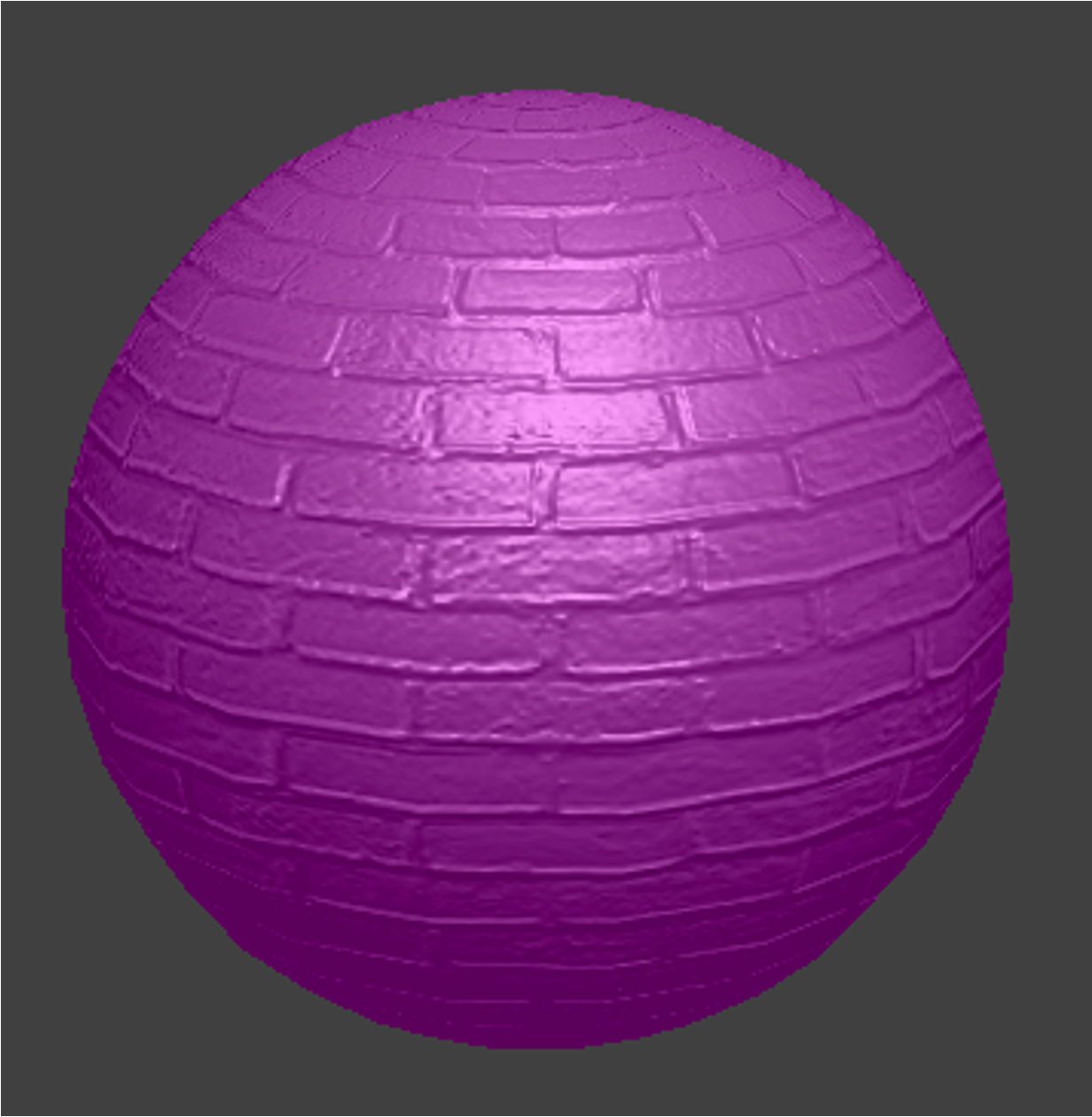
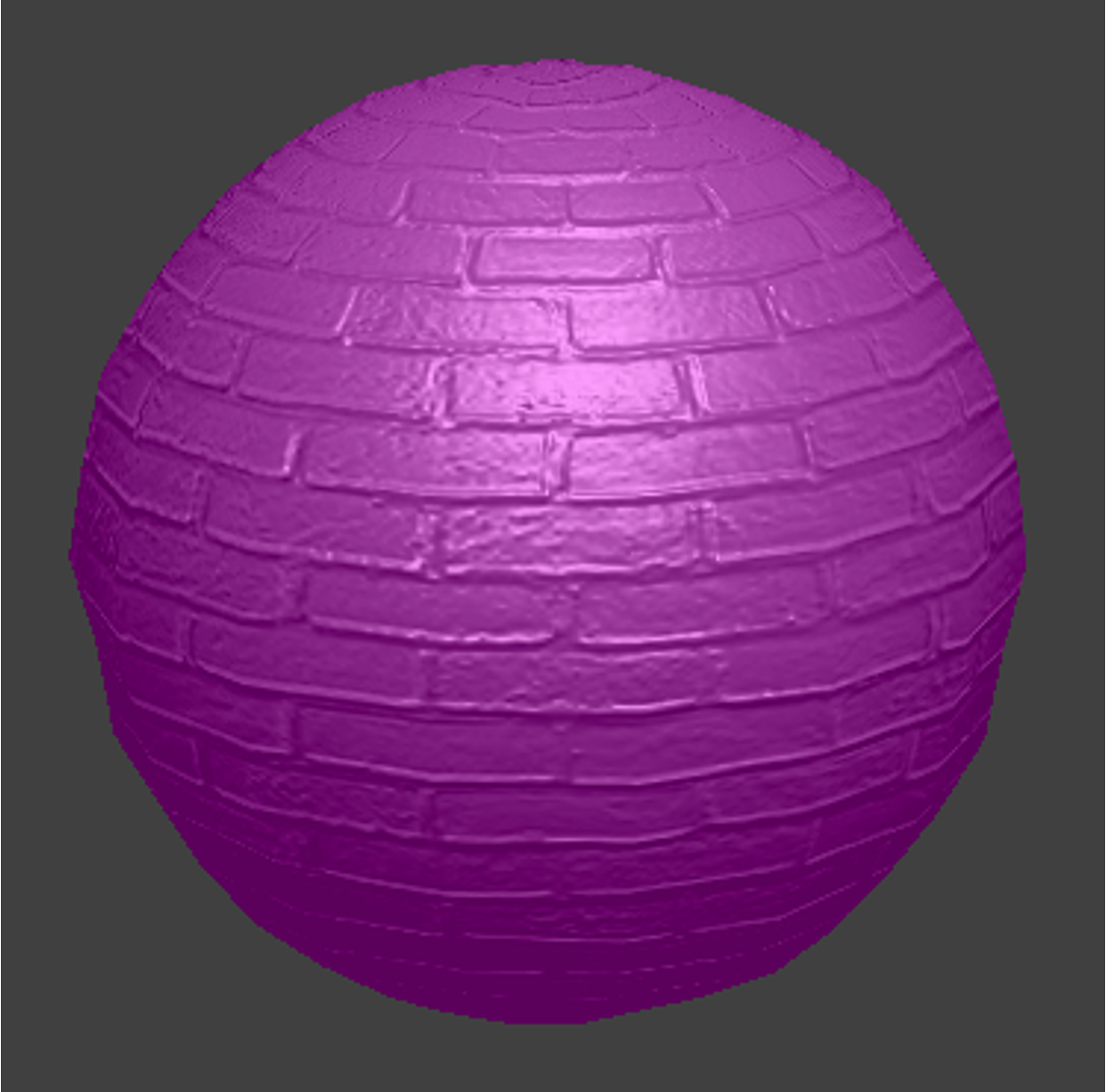
4. Bump and displacement mapping

Sphere with bump mapping	Sphere with displacement mapping
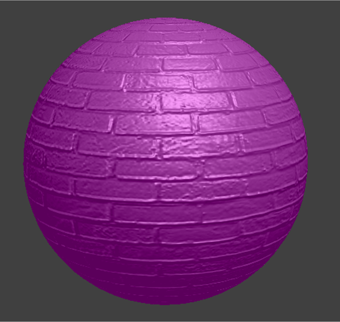Cloth with bump mapping	Cloth with displacement mapping

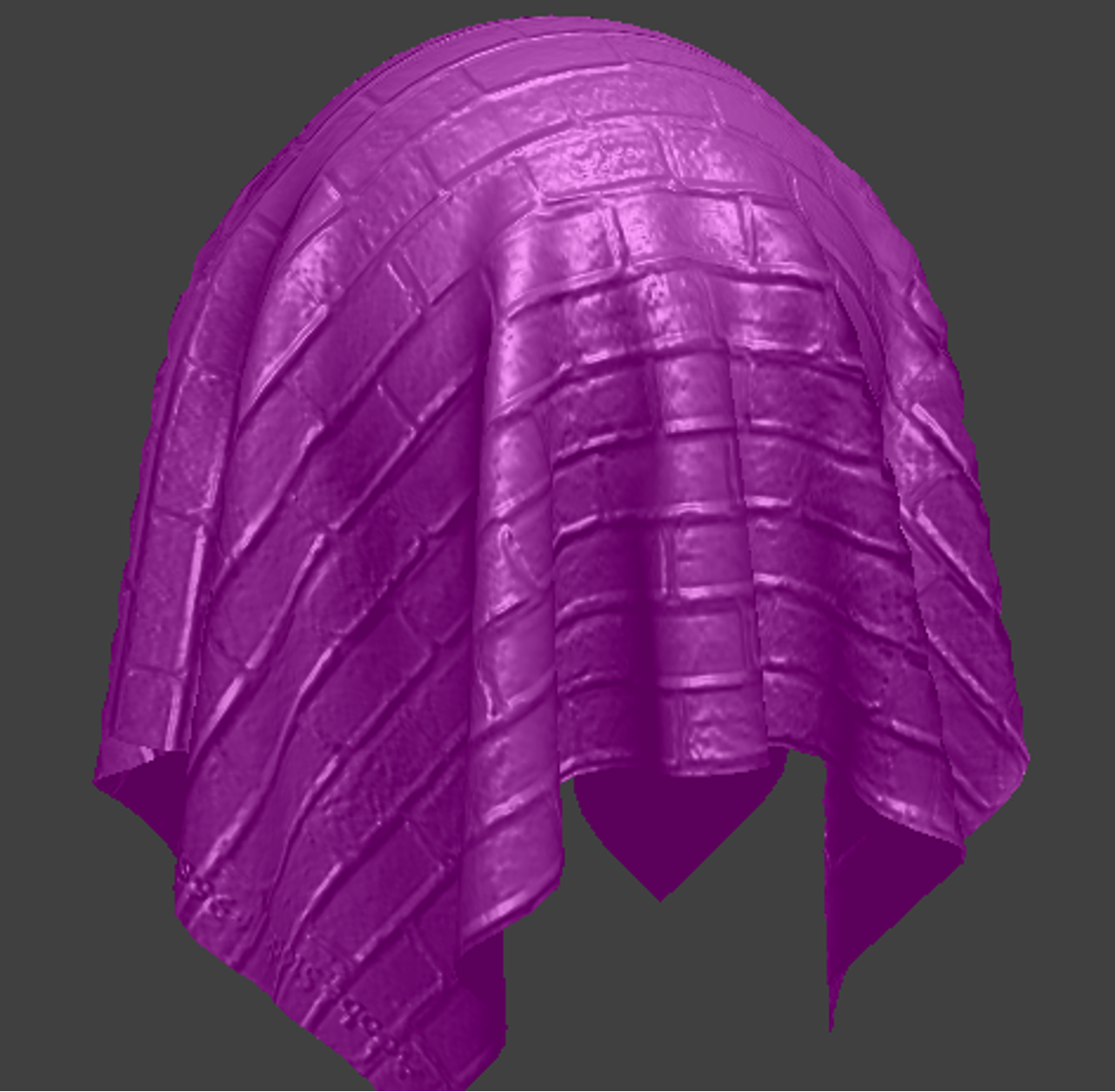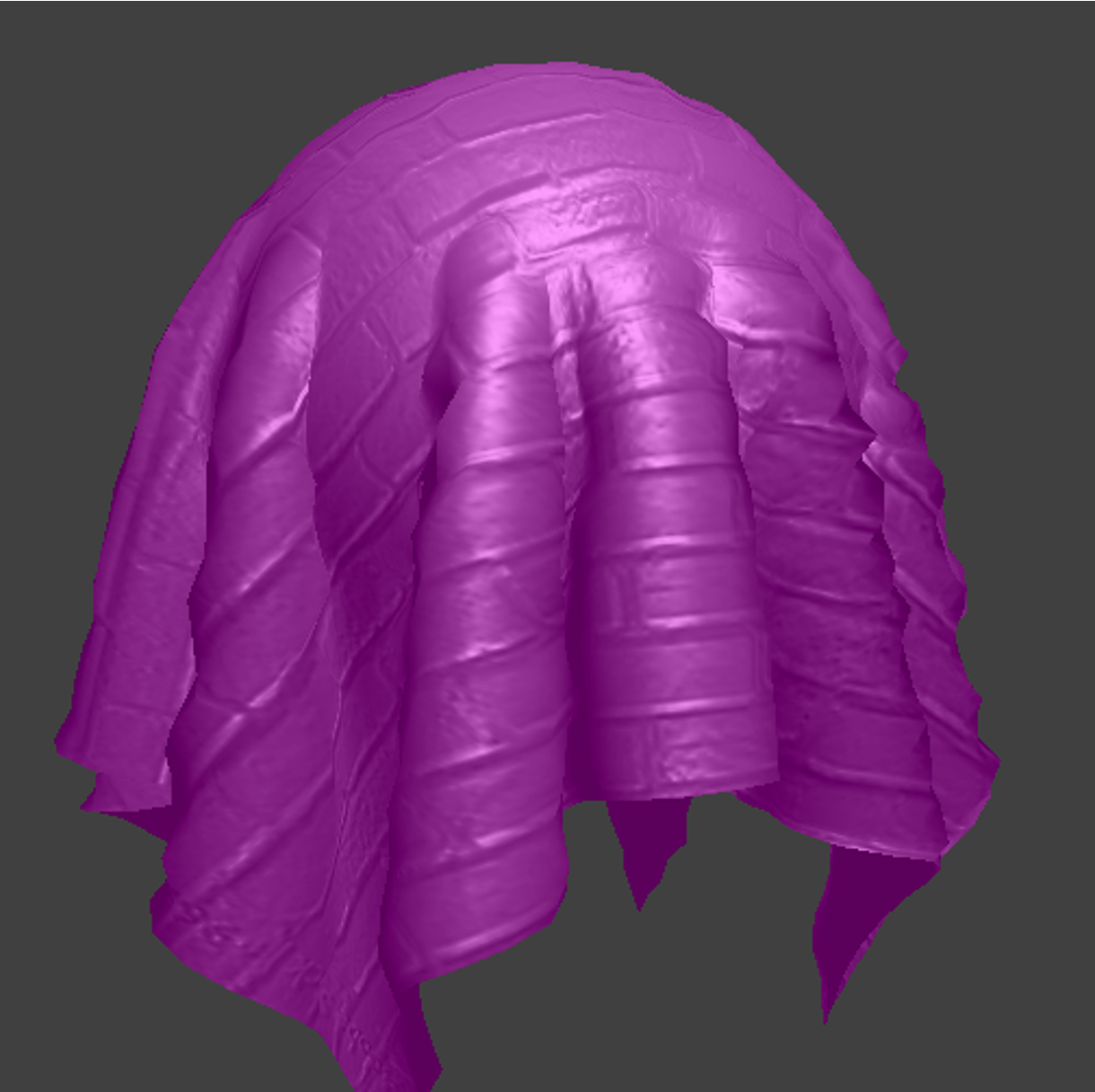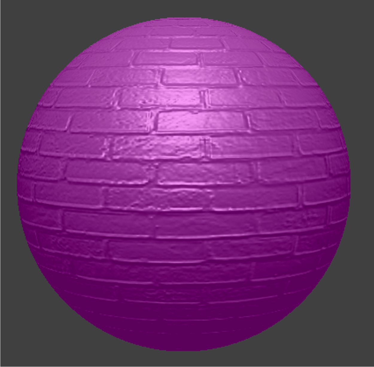
As we can see from the results, bump mapping transforms the local normal without modifying the actual mesh geometry, which gives us realistic reflection but relative fake mesh. In comparison, in addition to local normal transformation, displacement mapping also modify the textures of the mesh, giving more realistic visualization of the textures (e.g., intervals between the bricks).

Changing the sphere mesh’s coarseness

Sphere with bump mapping -o 16 -a 16	Sphere with displacement mapping -o 16 -a 16
Sphere with bump mapping -o 128 -a 128	Sphere with displacement mapping -o 128 -a 128

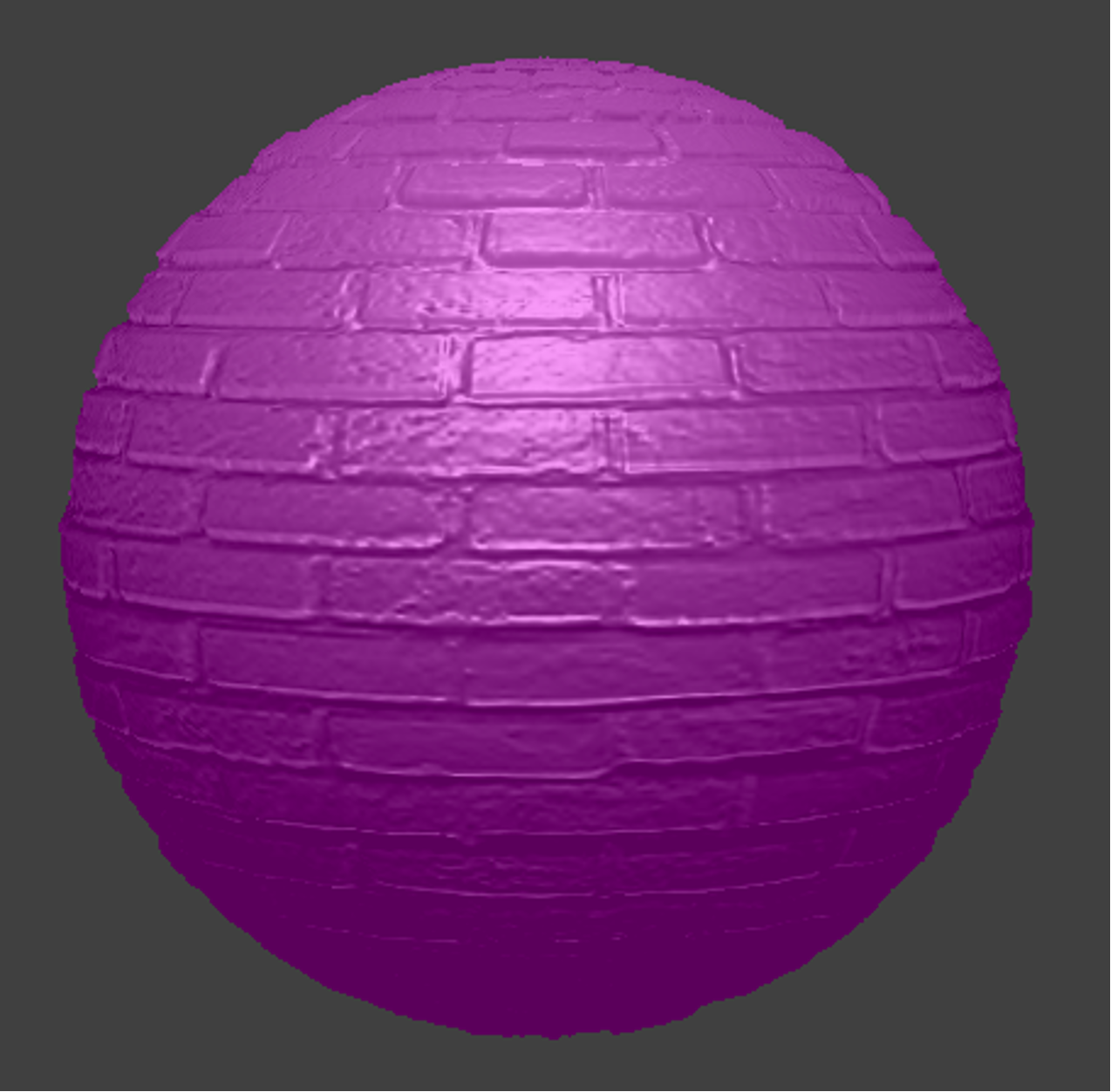As we can see from the results, higher coarseness gives sharper rendered textures. (e.g., intervals between the bricks)

5. Mirror shader

GIF for the simulation

In this task, we created a new cube environment-mapping using our cat photos from 6 directions (definitely far from perfect):

6. Extra Credit: Environment-mapped Displacement Mapping

Now, we want to add our cat’s textures to the displacement mapping! What we did is just sampling the light intensity term using the cube map:

vec3 intensity = texture(u_texture_cubemap,normalize(v)).rgb*4;

Our Custom.frag file looks like:

void main() {
  vec3 v_norm = normalize(v_normal.xyz);
  vec3 v_tang = normalize(v_tangent.xyz);
  vec3 b = cross(v_norm,v_tang);
  mat3 TBN = mat3(v_tang,b,v_norm);
  float dU = (h(vec2(v_uv.x + 1/u_texture_2_size.x,v_uv.y))-h(v_uv))*u_height_scaling*u_normal_scaling;
  float dV = (h(vec2(v_uv.x,v_uv.y+ 1/u_texture_2_size.y))-h(v_uv))*u_height_scaling*u_normal_scaling;
  vec3 n0 = vec3(-dU,-dV, 1);
  vec3 nd = TBN * n0;

  vec3 vnorm = normalize(nd);
  vec3 l= u_light_pos - v_position.xyz;
  vec3 v = u_cam_pos - v_position.xyz;
  vec3 intensity = texture(u_texture_cubemap,normalize(v)).rgb*4;


  vec3 h = normalize(normalize(l) + normalize(v));
  vec3 I_a = normalize(vec3(1,1,1));
  float k_a = 0.3;
  float k_d = 1;
  vec3 kd_term = k_d*(intensity/dot(l,l))*max(0,dot(vnorm,normalize(l)));
  float k_s = 0.8;
  float p = 20;
  vec3 ks_term = k_s*(intensity/dot(l,l))*pow(max(0,dot(vnorm,h)),p);
  // (Placeholder code. You will want to replace it.)
  vec3 L_total = k_a*I_a + kd_term + ks_term;
  out_color.rgb = L_total;
  out_color.a = 1;
}

Gif Animation GIF for the simulation

Part 6 - Extra Credit: Aerodynamic forces and wind simulation.

We implemented aerodynamic forces for wind simulation! To do so, we followed equations described here and here.

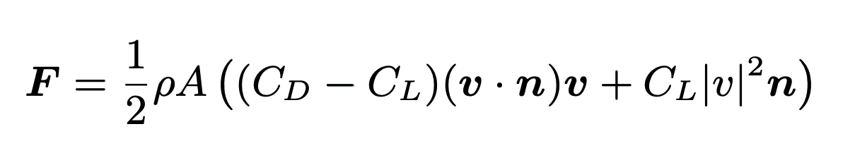
We also added a scaling coefficient term to enhance these forces. By following these aerodynamic equations, we obtain a different force at each position in the cloth that depends on: the cloth orientation (normal), point mass relative velocity to wind field, current area at point mass (area varies if cloth is stretched or not). In the equation: rho is the air density, A is the area at the point mass, C_D and C_L are the drag and lift coefficients, v is the relative speed with respect to the wind speed of the cloth at the point mass, and n is the cloth normal at the point mass position.

For simplicity, we simulated a constant wind field (i.e. wind speed is the same everywhere). However, in the future, we could modify this and include a 3D varying wind field map. We could treat this wind field map as a texture and extract the wind velocity at some coordinate based on the point mass position. Also, we could (and should) incorporate how objects alter the wind field map, which could potentially be done following Navier-Stokes equations like in smoke simulation.

The code to include aerodynamic forces, which was added to Cloth::simulate before Verlet integration, looks as follows:

  // Extra credit: aerodynamic forces

  bool ADD_AERODYNAMICS = true;

  if (ADD_AERODYNAMICS) {

    Vector3D wind_speed = Vector3D(0., 0., 30.);  // constant wind vector field (m/s)

    double rho = 1.225;  // air density from google
    double drag_coeff = 1.00;
    double lift_coeff = 0.5;  // drag_coeff >= lift_coeff
    double scale_coeff = 5.0;

    for (int row = 0; row < num_height_points; row++) {  // y coord
      for (int col = 0; col < num_width_points; col++) {  // x coord
        PointMass &pm = point_masses[row * num_width_points + col];

        // In edge case use neighbor to the other side to approximate normal
        Vector3D delta_row;
        Vector3D delta_col;
        if (row > 0) {
          delta_row = point_masses[(row - 1) * num_width_points + col].position - pm.position;
        } else {
          delta_row = pm.position - point_masses[(row + 1) * num_width_points + col].position;
        }
        if (col > 0) {
          delta_col = point_masses[row * num_width_points + (col - 1)].position - pm.position;
        } else {
          delta_col = pm.position - point_masses[row * num_width_points + (col + 1)].position;
        }

        Vector3D cross_prod = cross(delta_row, delta_col);
        double area = cross_prod.norm();
        Vector3D normal = cross_prod.unit();

        Vector3D relative_velocity = (pm.position - pm.last_position) / delta_t - wind_speed;
        normal = (dot(normal, relative_velocity) > 0) ? normal : -normal;

        Vector3D wind_force = (drag_coeff - lift_coeff) * dot(relative_velocity, normal) * relative_velocity;
        wind_force += lift_coeff * relative_velocity.norm2() * normal;
        wind_force *= 0.5 * rho * area;

        pm.forces -= scale_coeff * wind_force;
      }
    }
  }

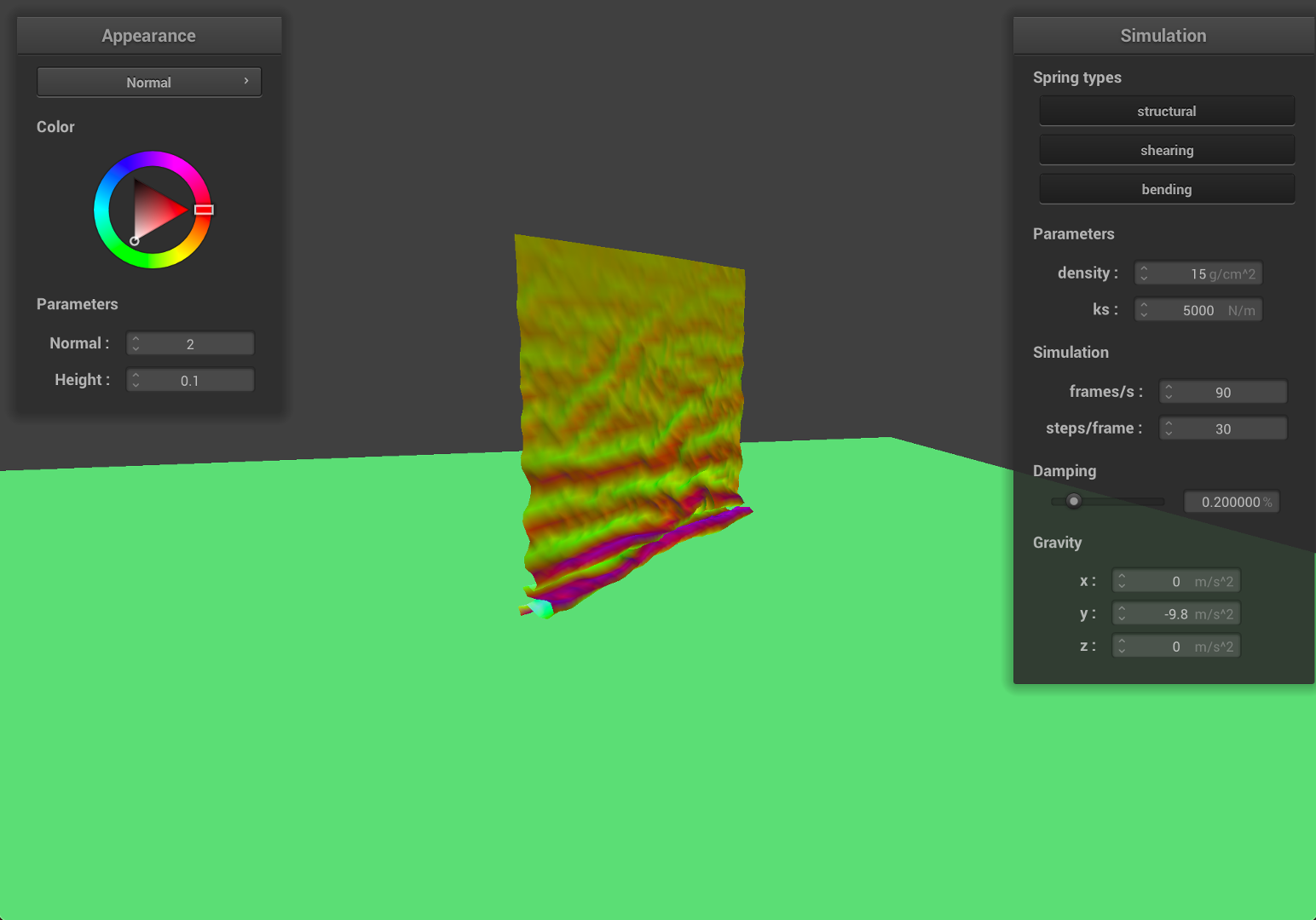
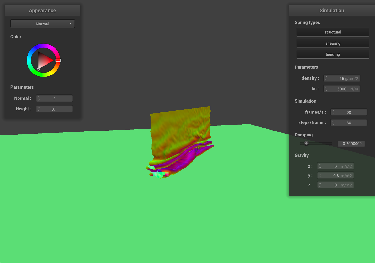
The results are super cool! We can also note that these aerodynamic forces also play a role even if there’s no wind: if the cloth has some speed, then there will be aerodynamic forces which will slow it down. Below we show some cool examples where we simulated wind for some pinned cloths:

Vertical cloth with 2 vertices pinned:

Vertical cloth with all 4 vertices pinned:

Note on collaboration

We’ve been working together since the first project, as well as collaborating in research in our lab. For the CS284A course projects we’ve worked independently on the each task of the coding part of the assignment (in separate branches), and we would discuss issues / point out bugs / discuss alternative implementations. At the end we would either merge one of the two branches into master or combine parts of each branch. Now, for the write-up, we usually split the tasks. This has been working since we both have tight schedules and allows both of us to dig into the code (and learn in this process).