Overview
In this project, we simulate cloth. First, we build the cloth as a system of masses and springs connecting them.
Then, we add force and update the masses position according to the force acting on them. We also handle collision of the cloth on plane and shere as well as self-collision.
In the end, we add different shading to the cloth. We find the last part interesting and challenging because it is visually appealing.
Part I: Masses and springs
For this part, we need to fill the Cloth::buildGrid() function. First, we create num_height_points * num_width_points number of masses.
If the orientation of the cloth is vertical, we set position to (x: (point number on width side - 1 ) * width between 2 points, y: 1, z: (point number on height side - 1 ) * height between 2 points).
Then, loop through pinned vector. If the current pair of index is in the vector, the pinned is true for the mass.
If the orientation of the cloth is horizontal, process is exactly the same as the above, but change the position to (x: (point number on width side - 1 ) * width between 2 points, y: (point number on height side - 1 ) * height between 2 points, z: random offset between -1/1000 and 1/1000).
Append each masses to point_masses vector.
In the end, we add springs according to the rule on the spec:
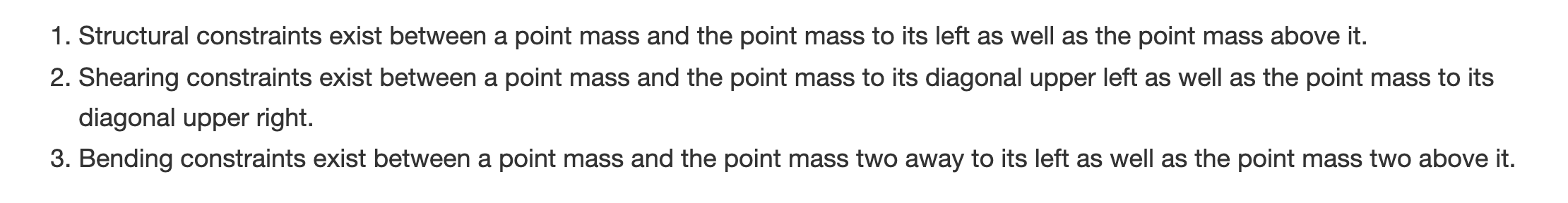 Spring adding rule.
|
We ensure edges are correct by checking that going left, right, above, below the current mass does not exceed the bounds (0, num_height_points - 1) and (0, num_width_points - 1).
Below pictures shows the masses and springs:
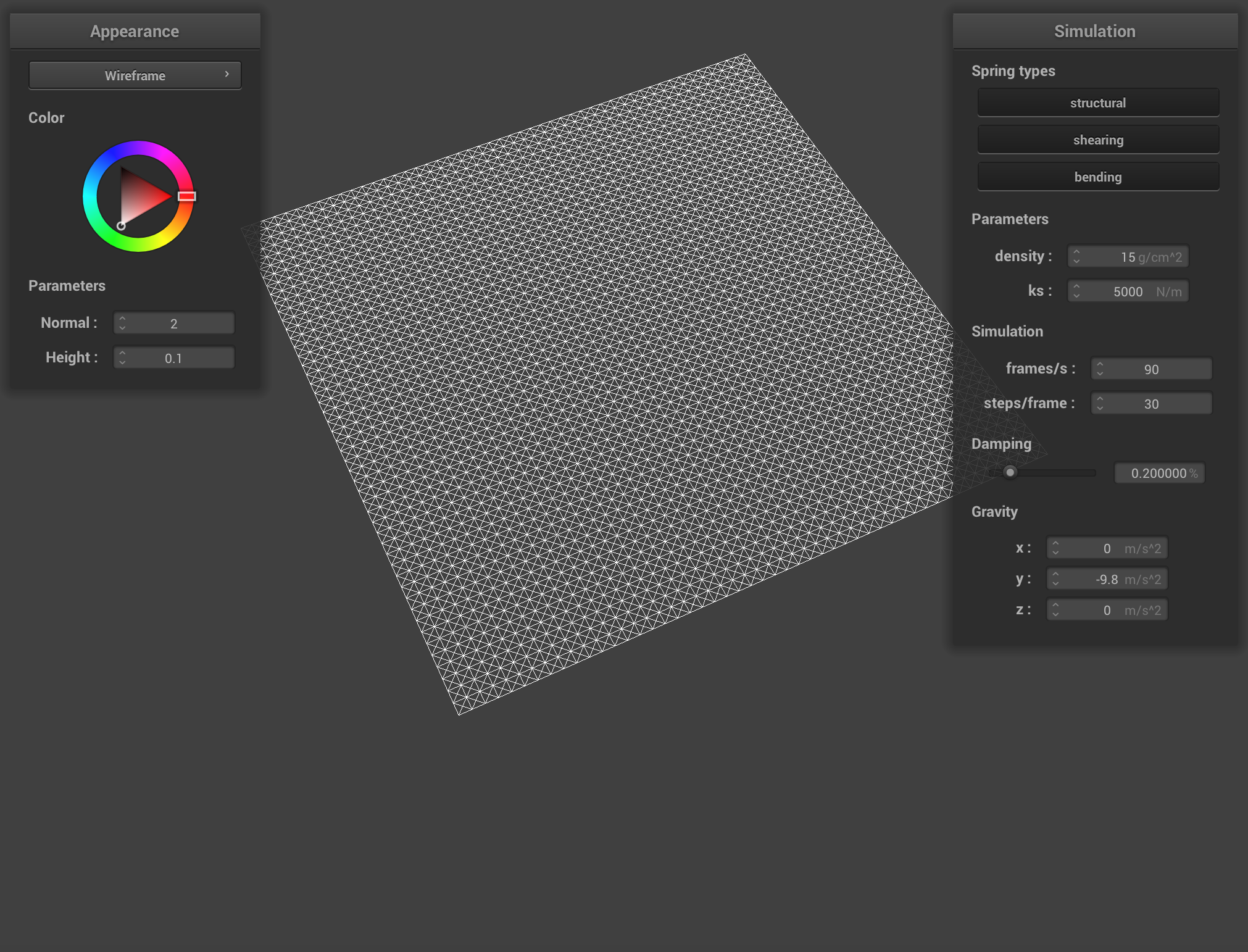
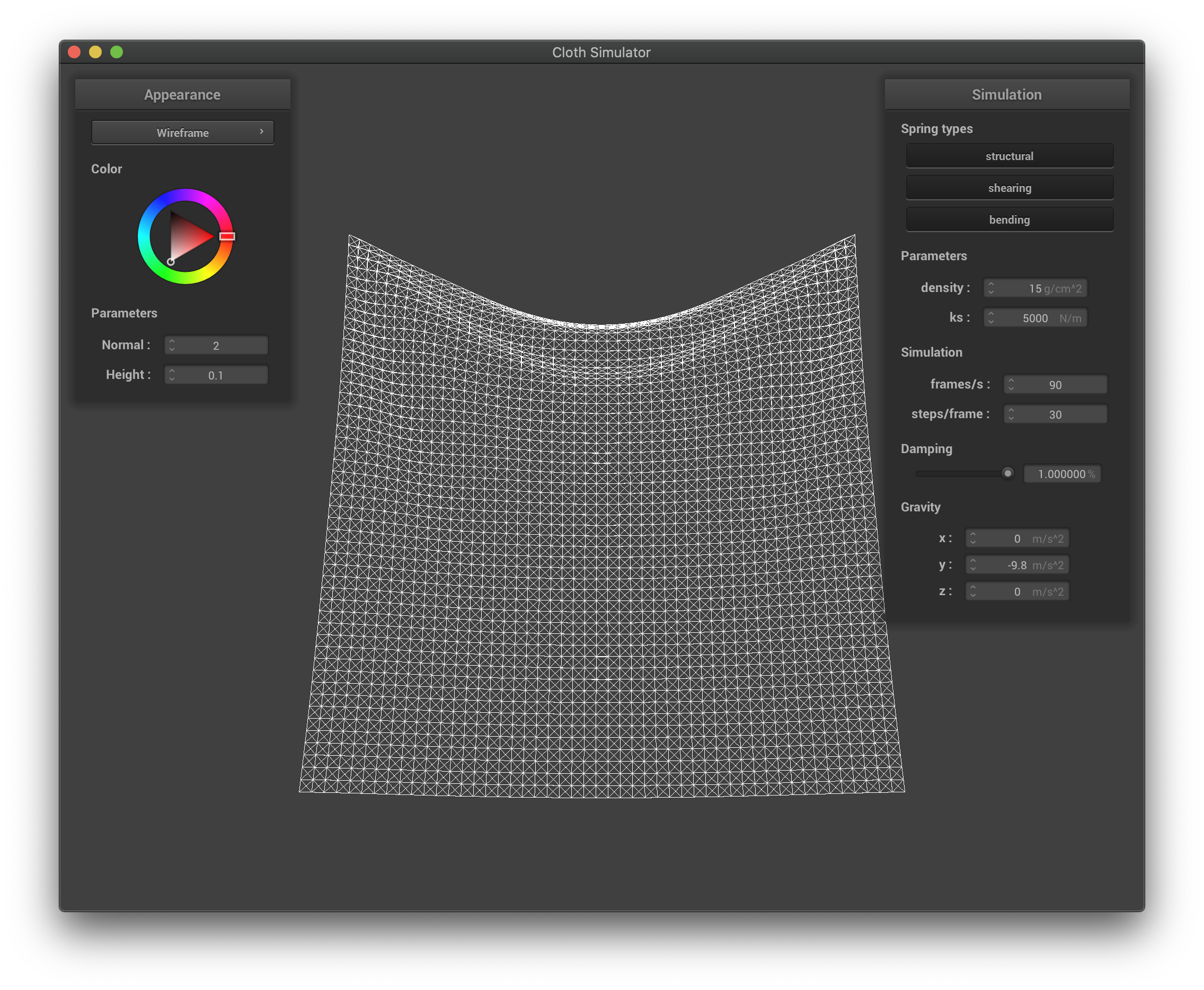
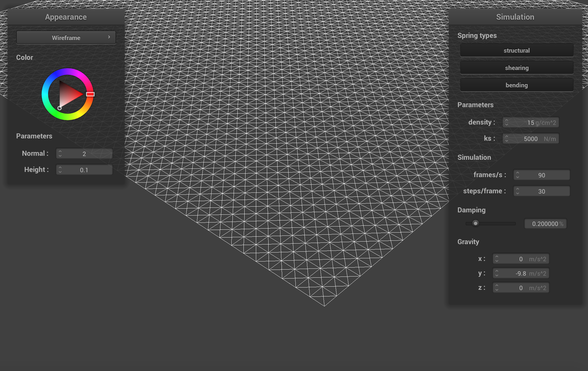 Some screenshots of scene/pinned2.json from a viewing angle where we can clearly see the cloth wireframe to show the structure of your point masses and springs.
|
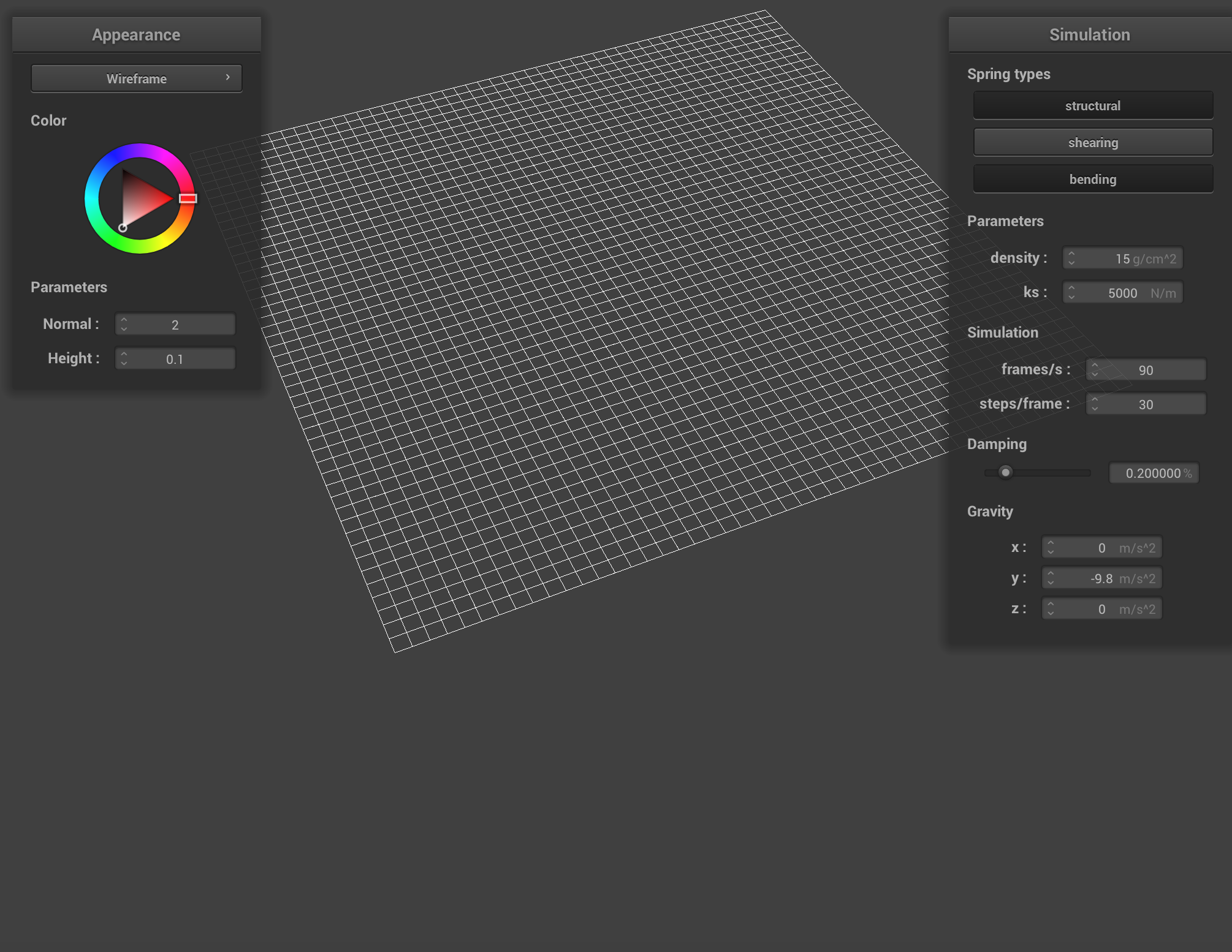 The wireframe (1) without any shearing constraints.
|
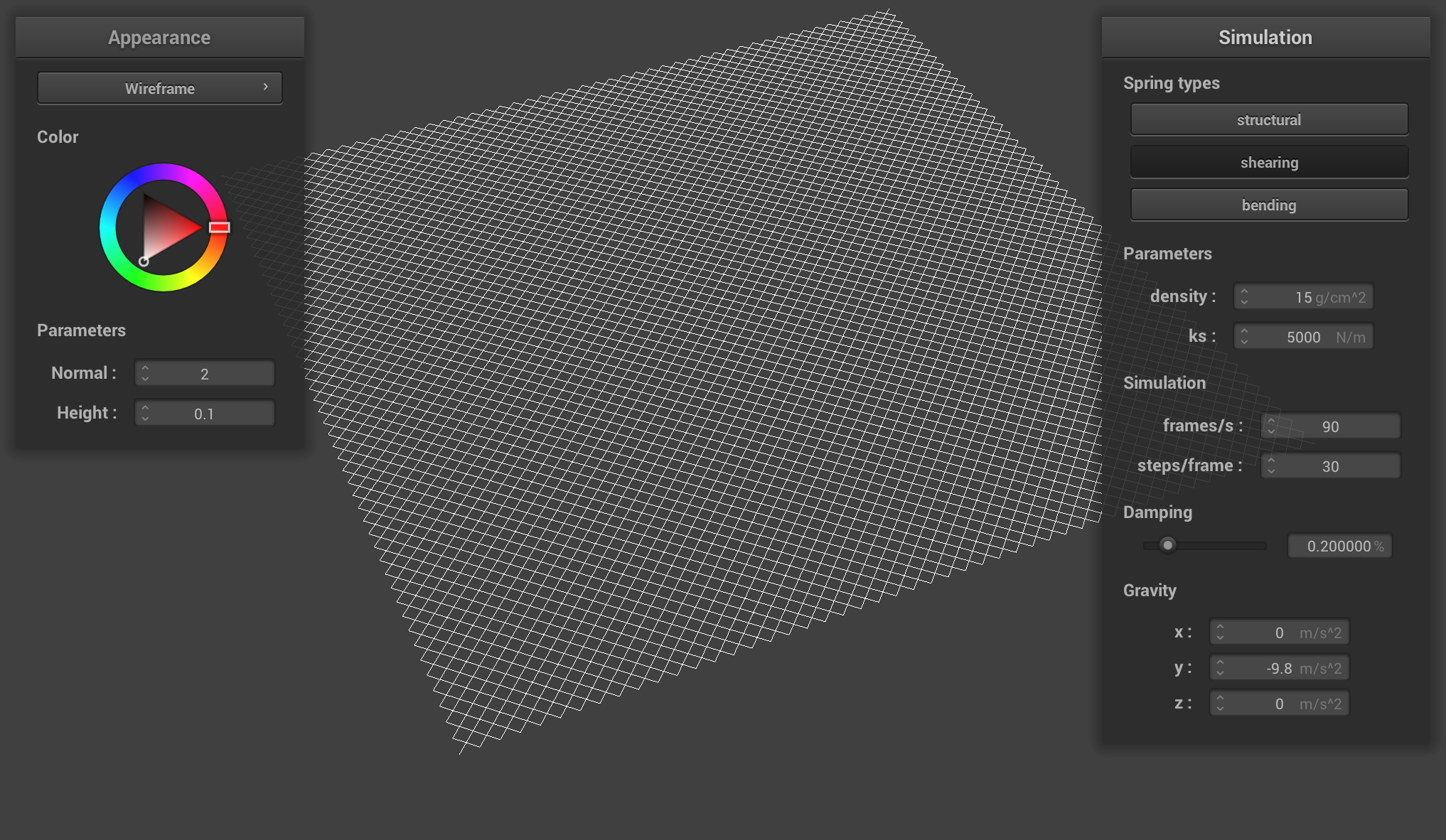 The wireframe (2) with only shearing constraints.
|
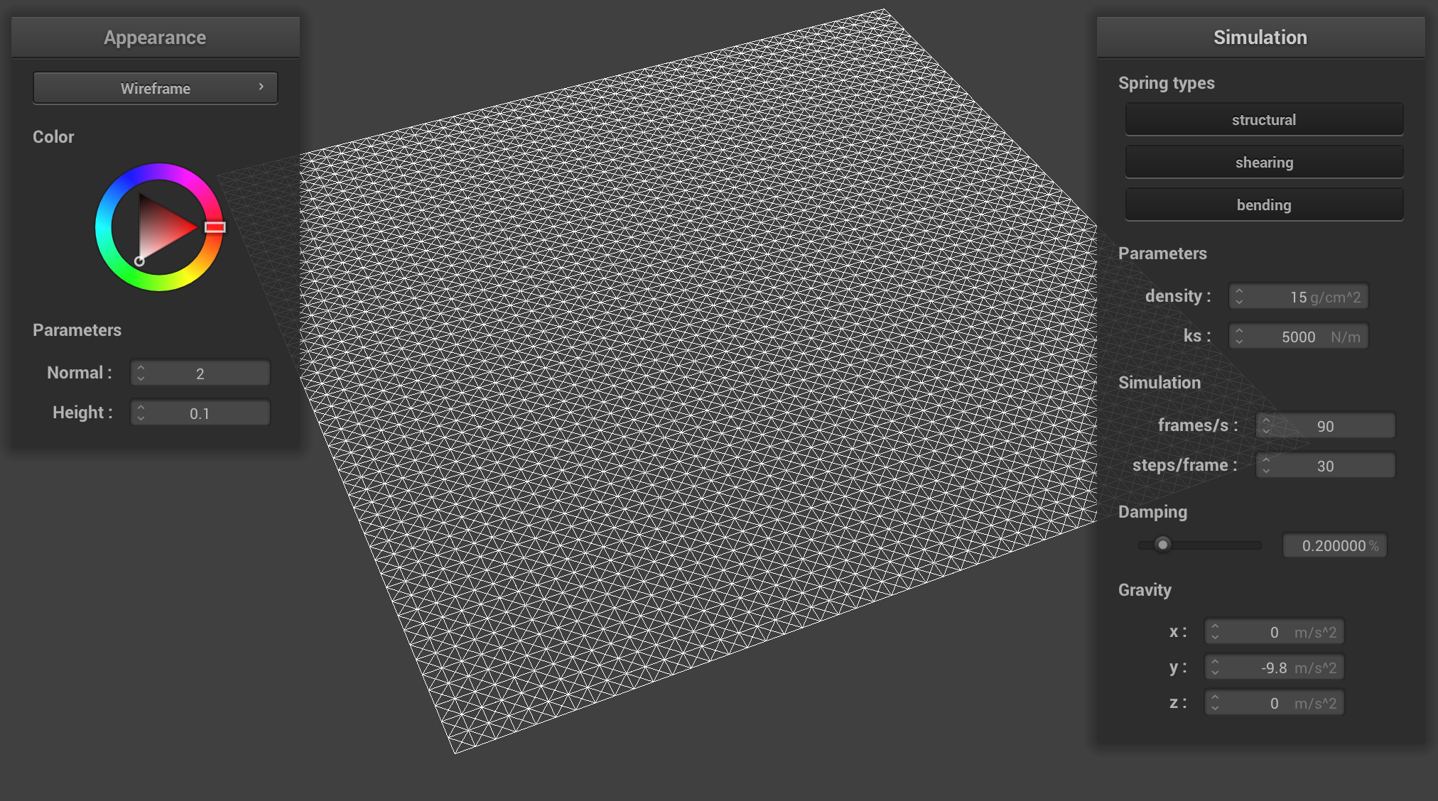 The wireframe (3) with all constraints.
|
Part II: Simulation via numerical integration
To implement simulation via numerical integration, we need to understand the basic physics behind the simulation.
First, we need to compute the total force acting on each point mass. There are two types of forces we will be simulating, which will be based on acceleration and springs. We need to calculate the total external force on each PointMass based on the external_accelerations and the mass using Newton’s 2nd Law. Then, we also need to apply the spring correction forces following the Hooke’s Law. We need to check it the spring’s constraint type is enabled, and apply a bending factor of 0.2 if the spring is of bending type when calculating the force. Then, we apply the force on the two ends of the spring with the correct direction.
Then, we use Verlet integration to compute the new point mass positions, including a damping factor to account for other forces that are not in our simulation. We proceed to update the last_position and position for each point mass accordingly.
Another important part is that we need to add constraints to the springs so that they will behave more realistically in the simulation: the spring must be at most 10% more than its rest_length, or at most 10% less than its rest_length. If the current simulation violates this constraint, we need to adjust the end points of the springs to account for this using the midpoint of the spring as reference and set up the endpoints accordingly. We also need to be careful about the cases where the end points of the springs may be pinned, where we need to adjust one end point’s position according to the other pinned end point’s position.
Now, we have a working physics simulation.
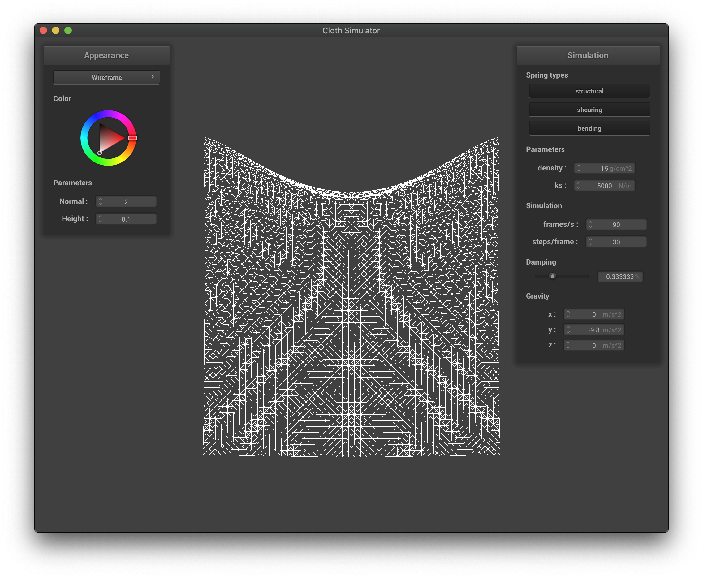
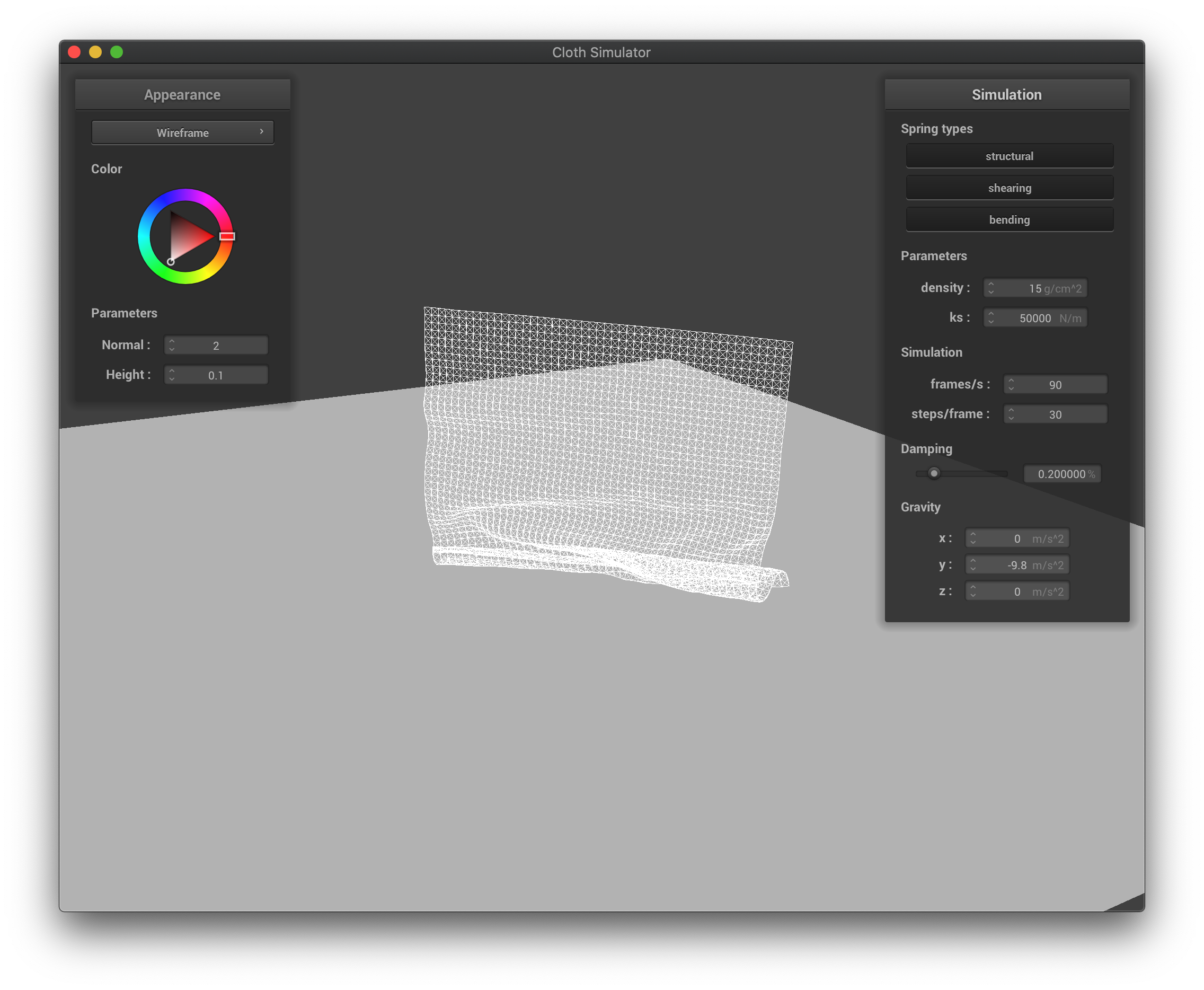
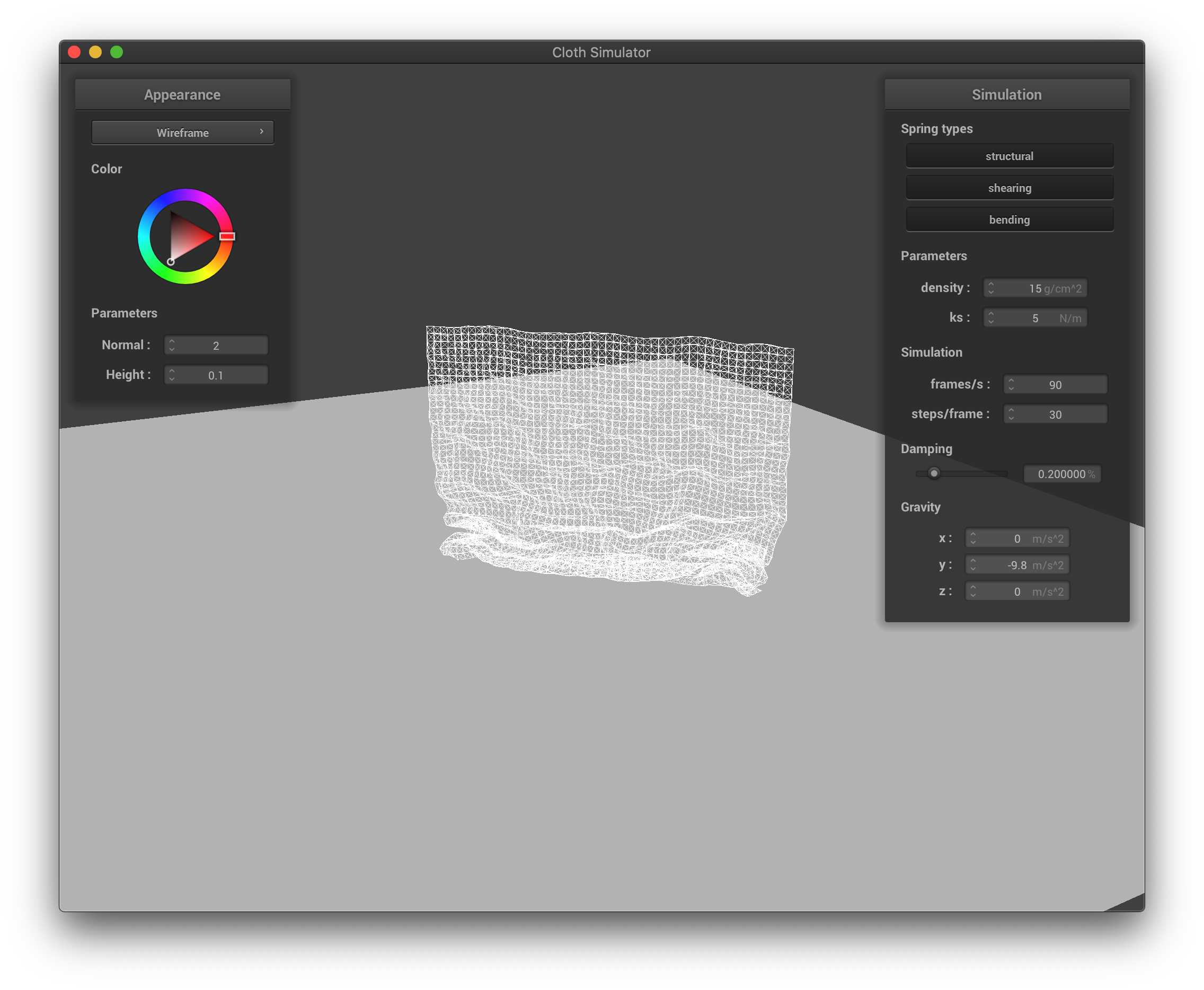
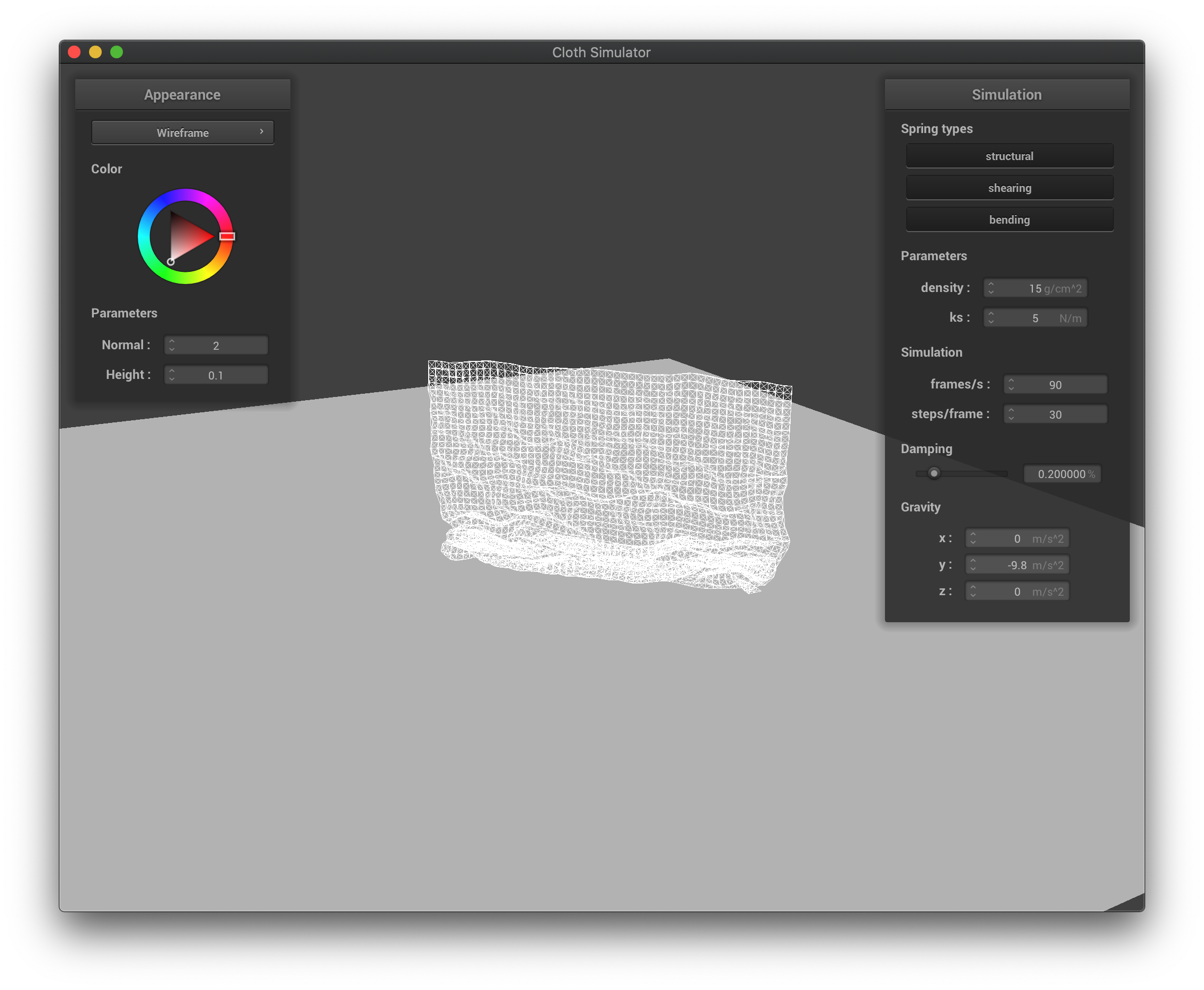
The spring constant reflects the stiffness of the spring, which in turn reflects how much force is generated given the change of length from the resting length. Changing this constant will in turn change the characteristic of the springs: if the spring constant is low, the cloth behaves very soft, bounces more, there could be multiple wrinkles on the cloth, and the top of the cloth has a larger concavity; if the spring constant is high, the cloth behaves much harder, bounces less, the top of the cloth has a smaller concavity, and the cloth is much flatter.
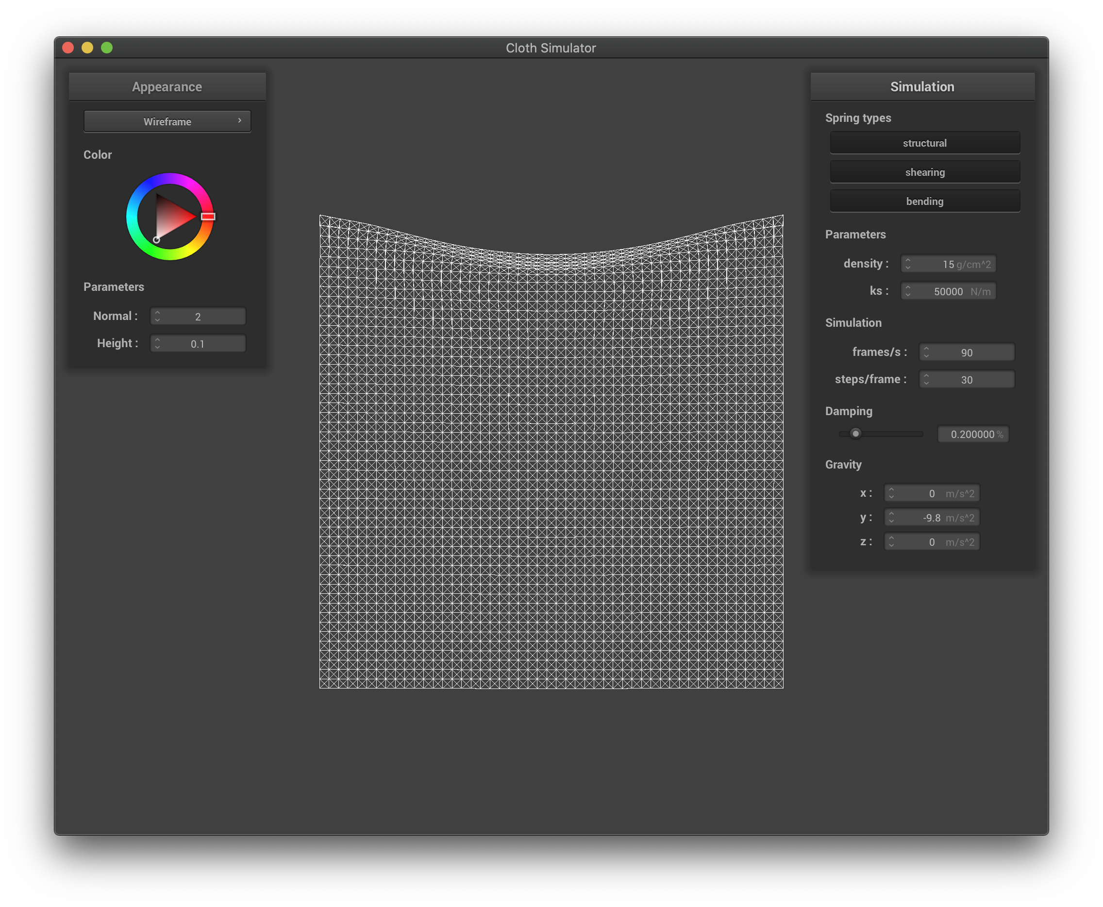 The wireframe with high spring constant.
|
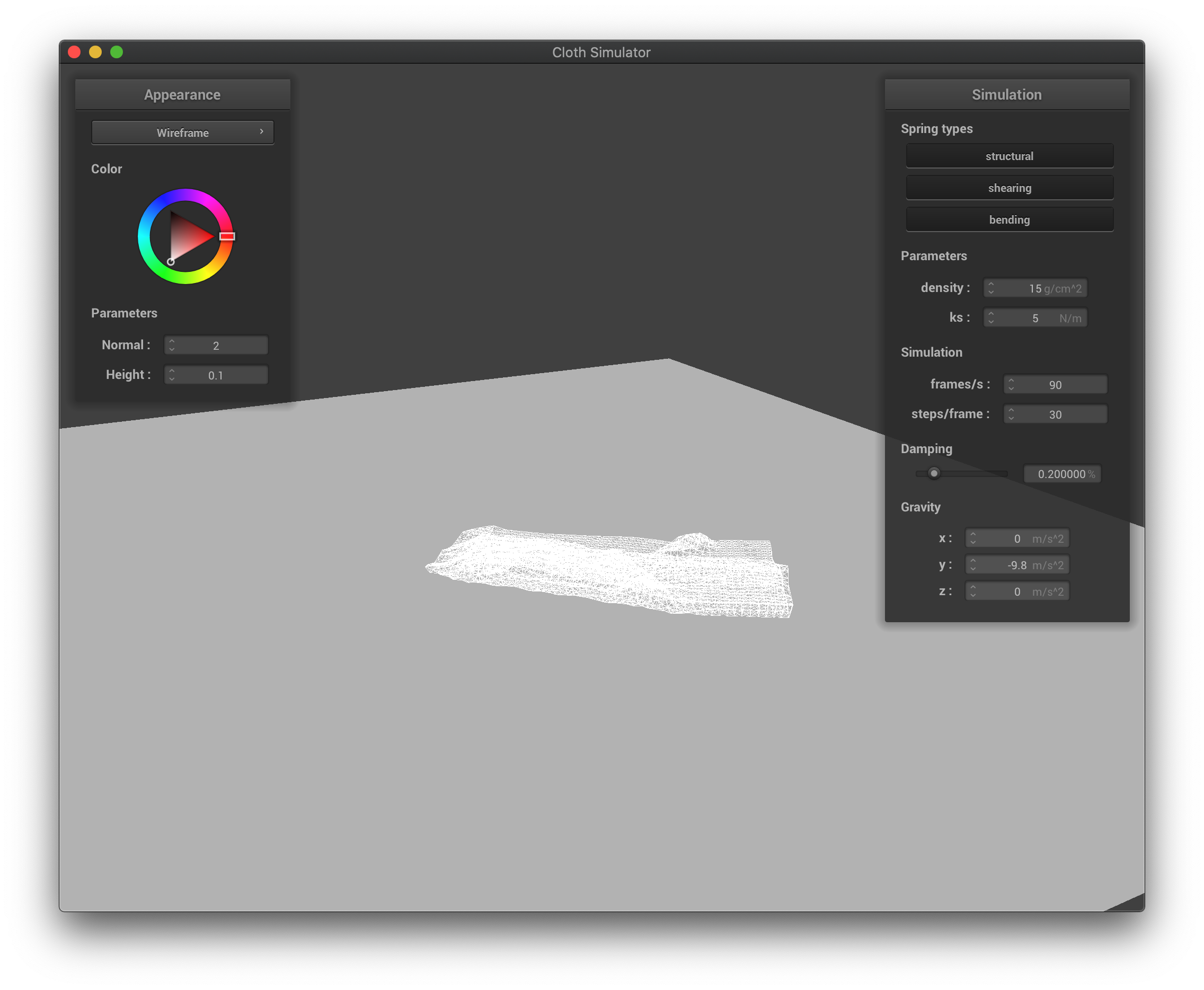
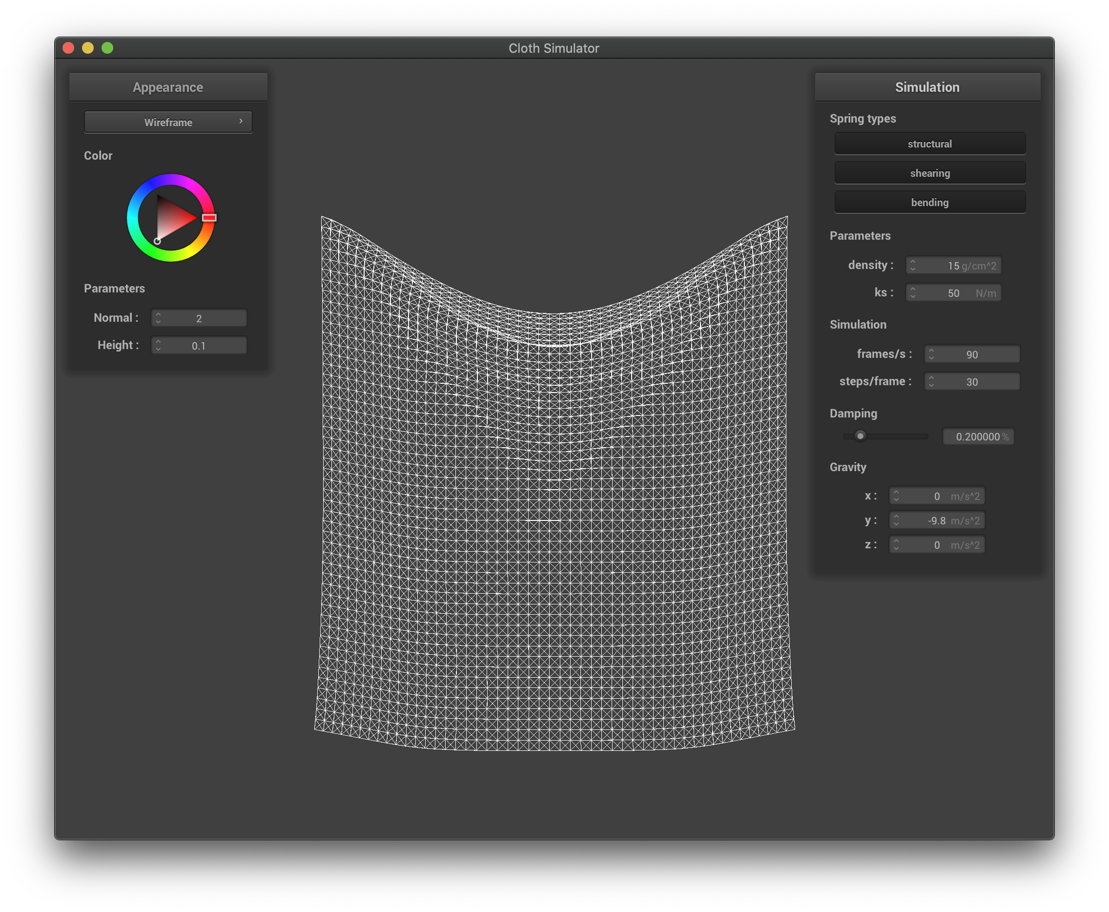 The wireframe with low spring constant.
|
The density affects the overall weight of the cloth, and by definition the weight per unit volume. If the density is higher, the cloth acts heavier, the top of the cloth has a larger deformation, and is stretched out more due to the extra weight; if the density is smaller, the cloth acts lighter, the top of the cloth has a smaller deformation, and is stretched out less since the weight is very small.
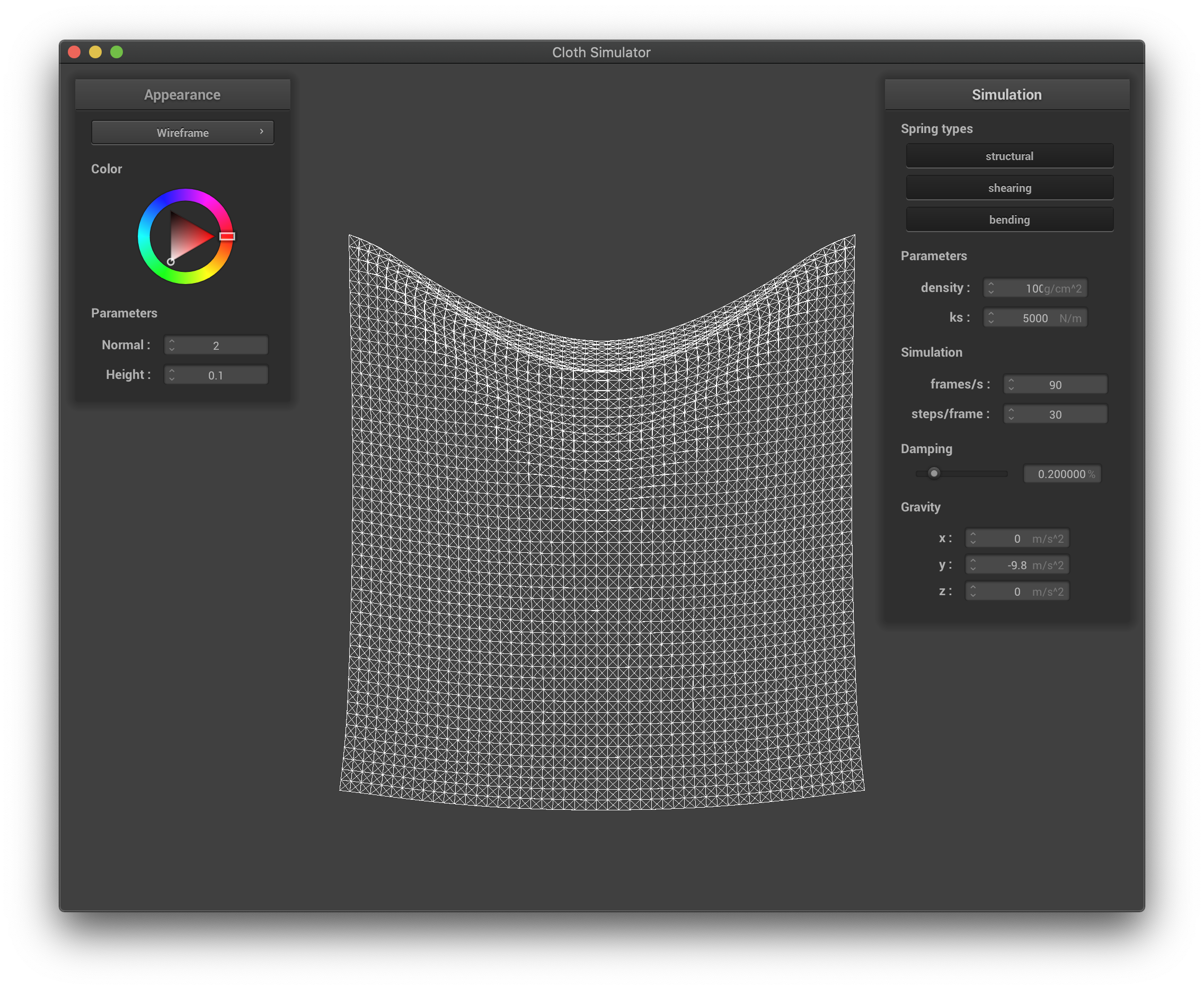 The wireframe with high density.
|
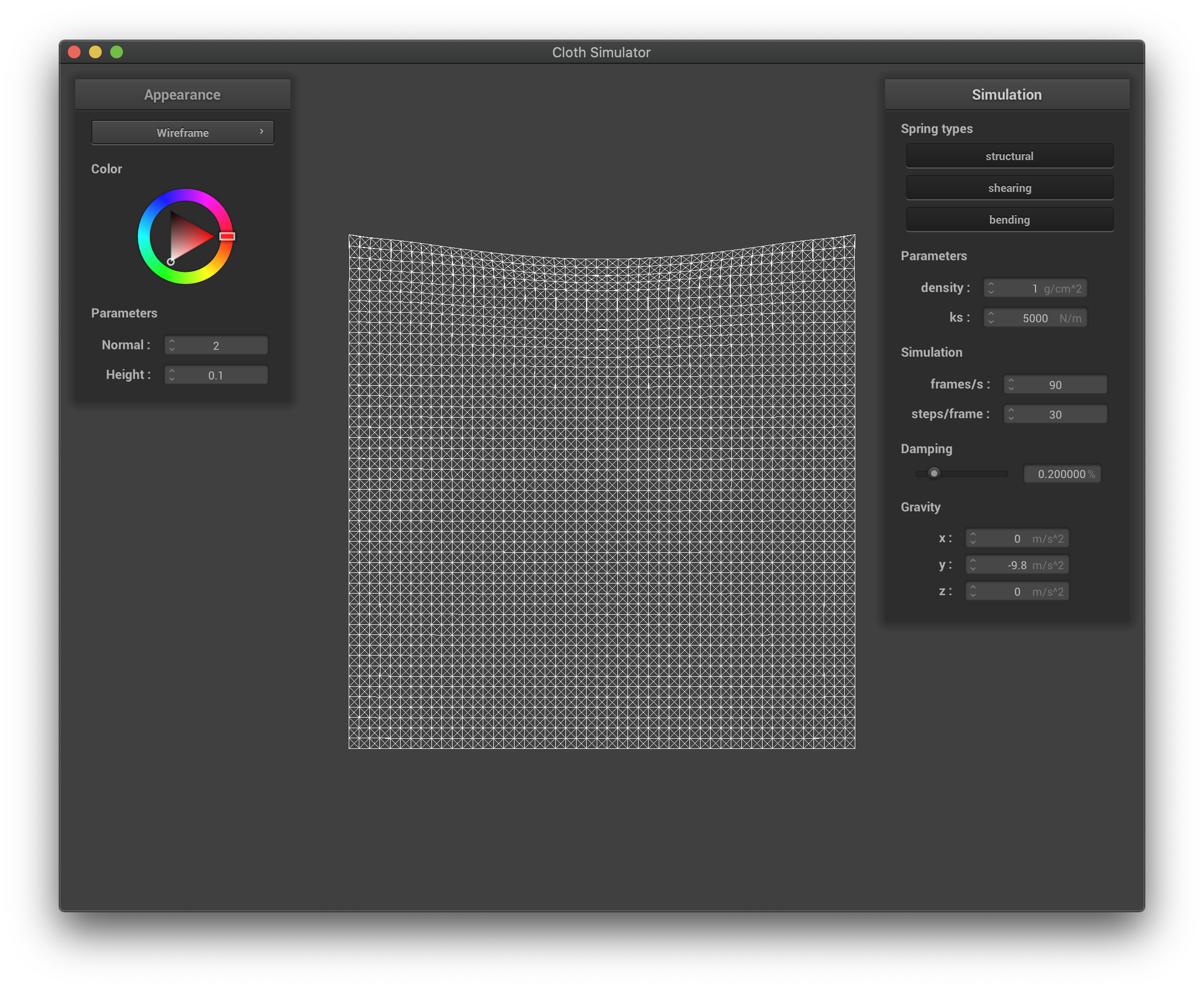 The wireframe with low density.
|
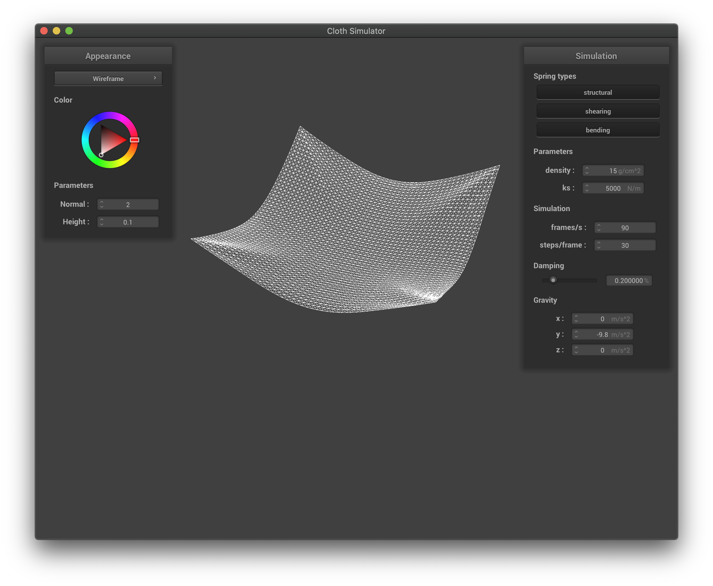
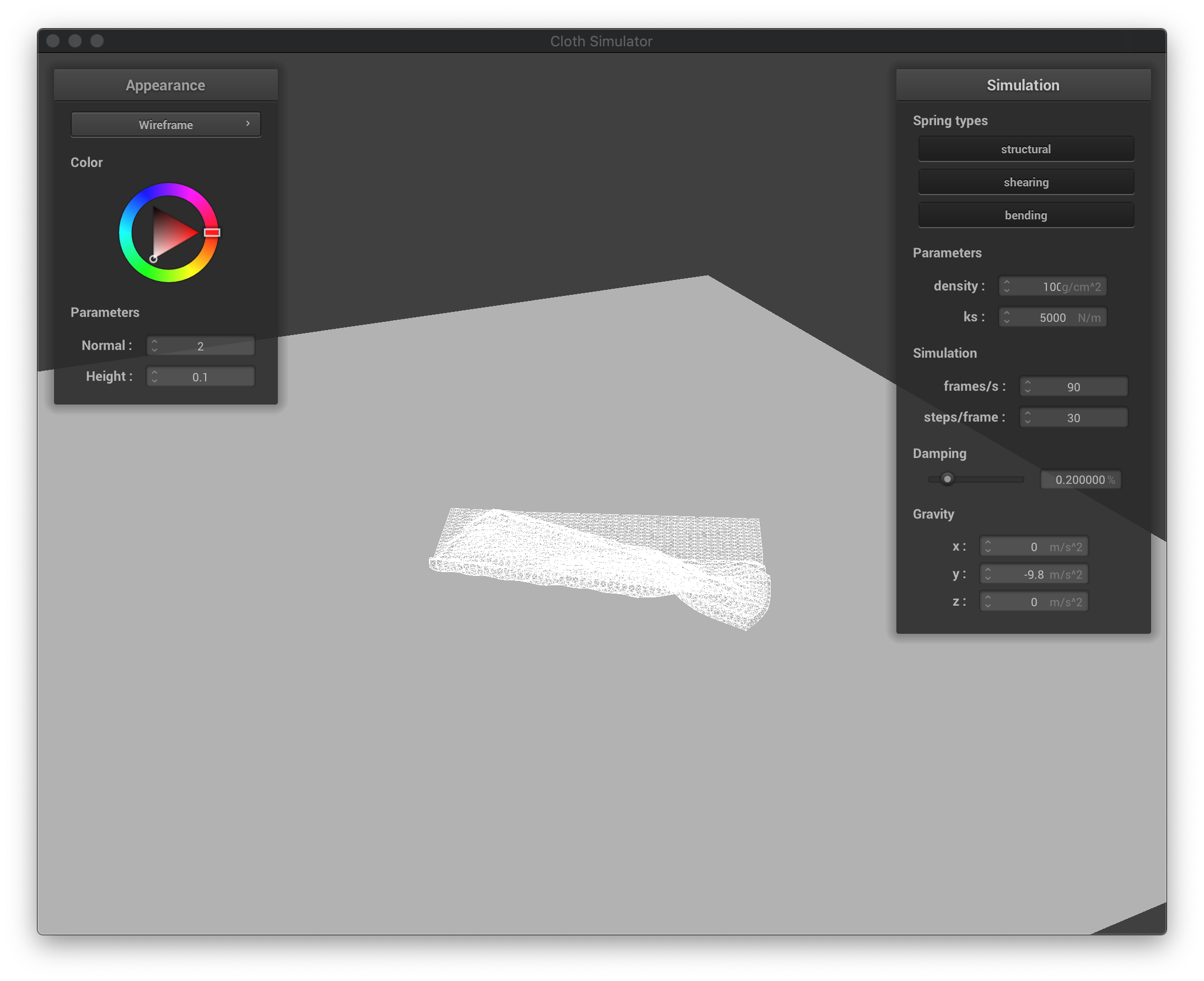
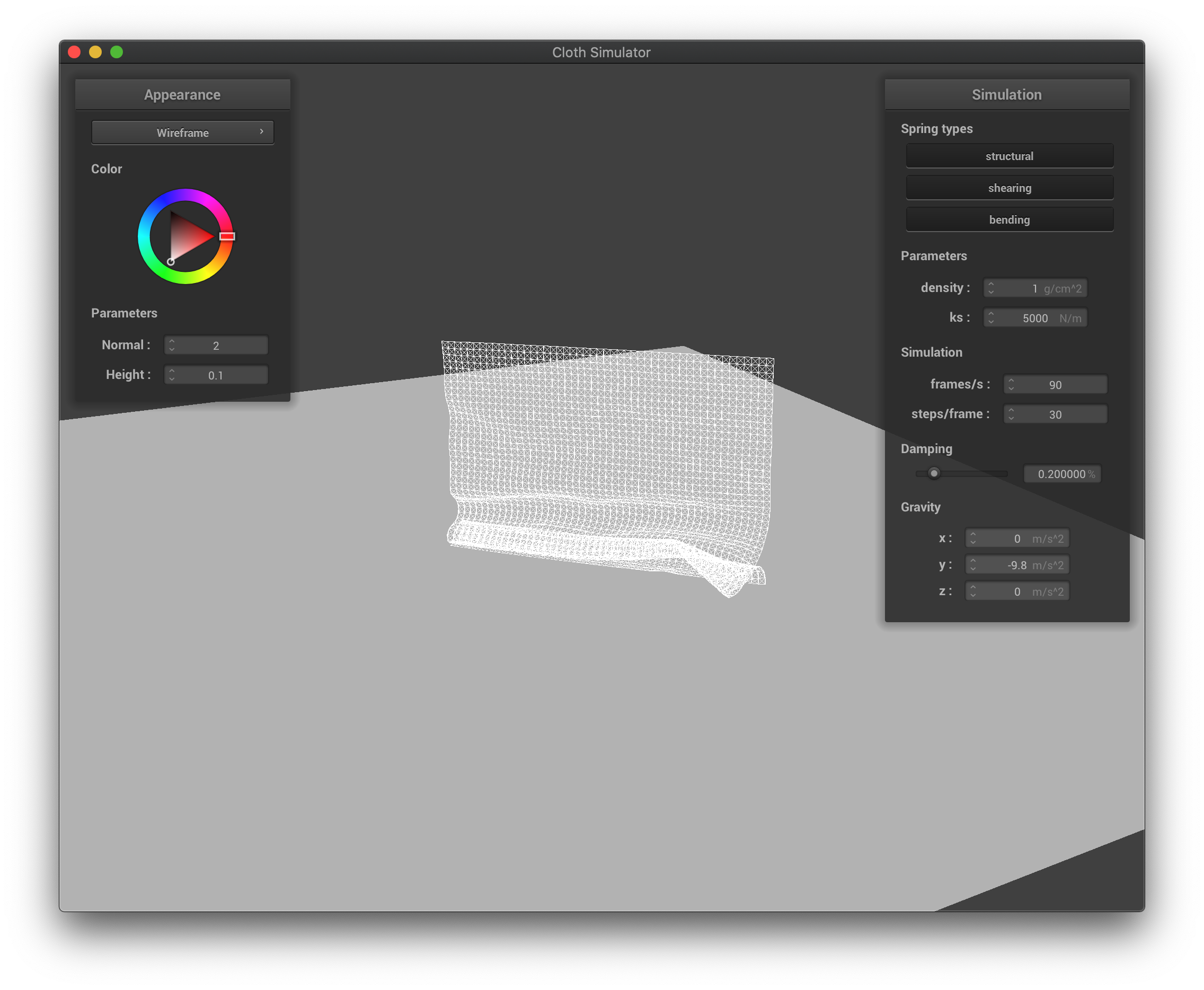
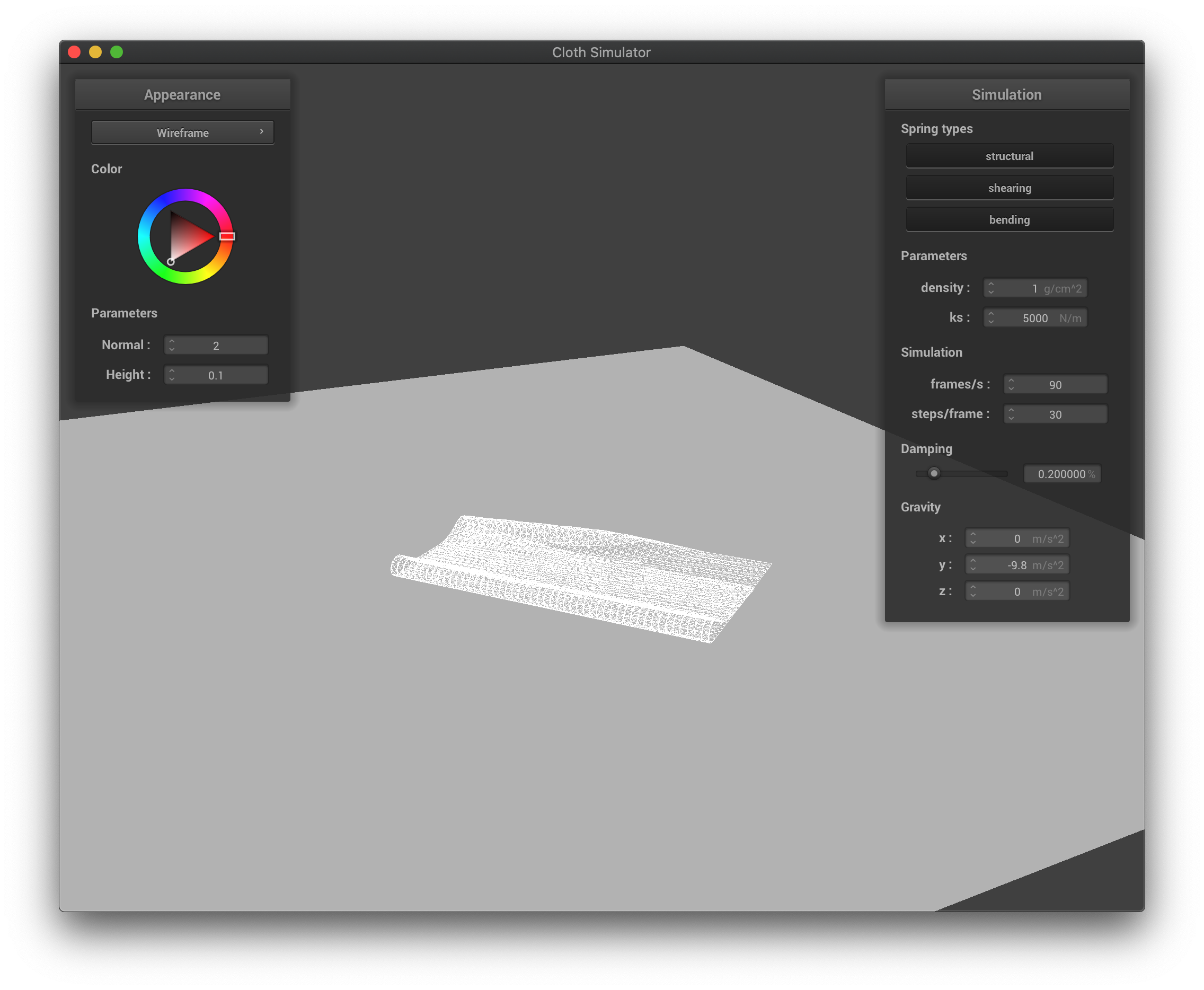
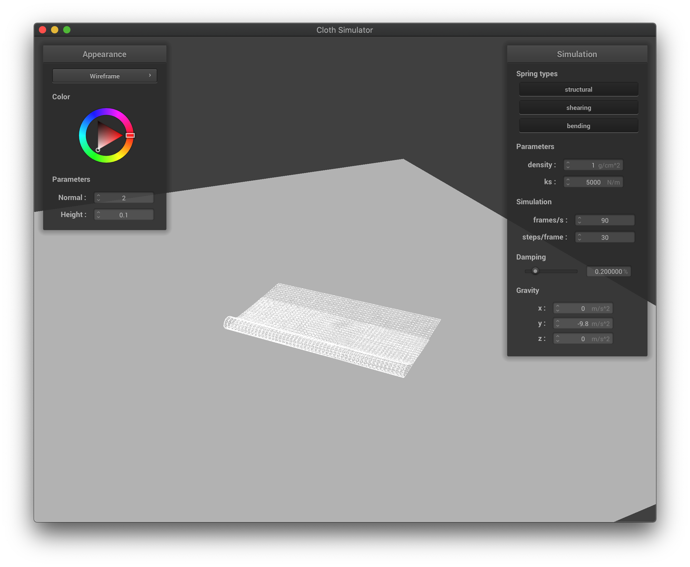
The damping constant characterizes the external drags caused by the environment. It in turn affects the falling speed of the cloth, as well as how much the cloth bounces before coming to a stable state. If this constant is larger, the cloth falls much slower, and it exhibits fewer oscillations once becoming vertical; if this constant is smaller, then the cloth falls much quicker, and it bounces more before coming to a complete stable state (or never if the constant is zero, as the forces will act on each point mass forever). We present images taken at similar time stamps as the simulation started:
 The wireframe with very high damping factor.
|
 The wireframe with high damping factor.
|
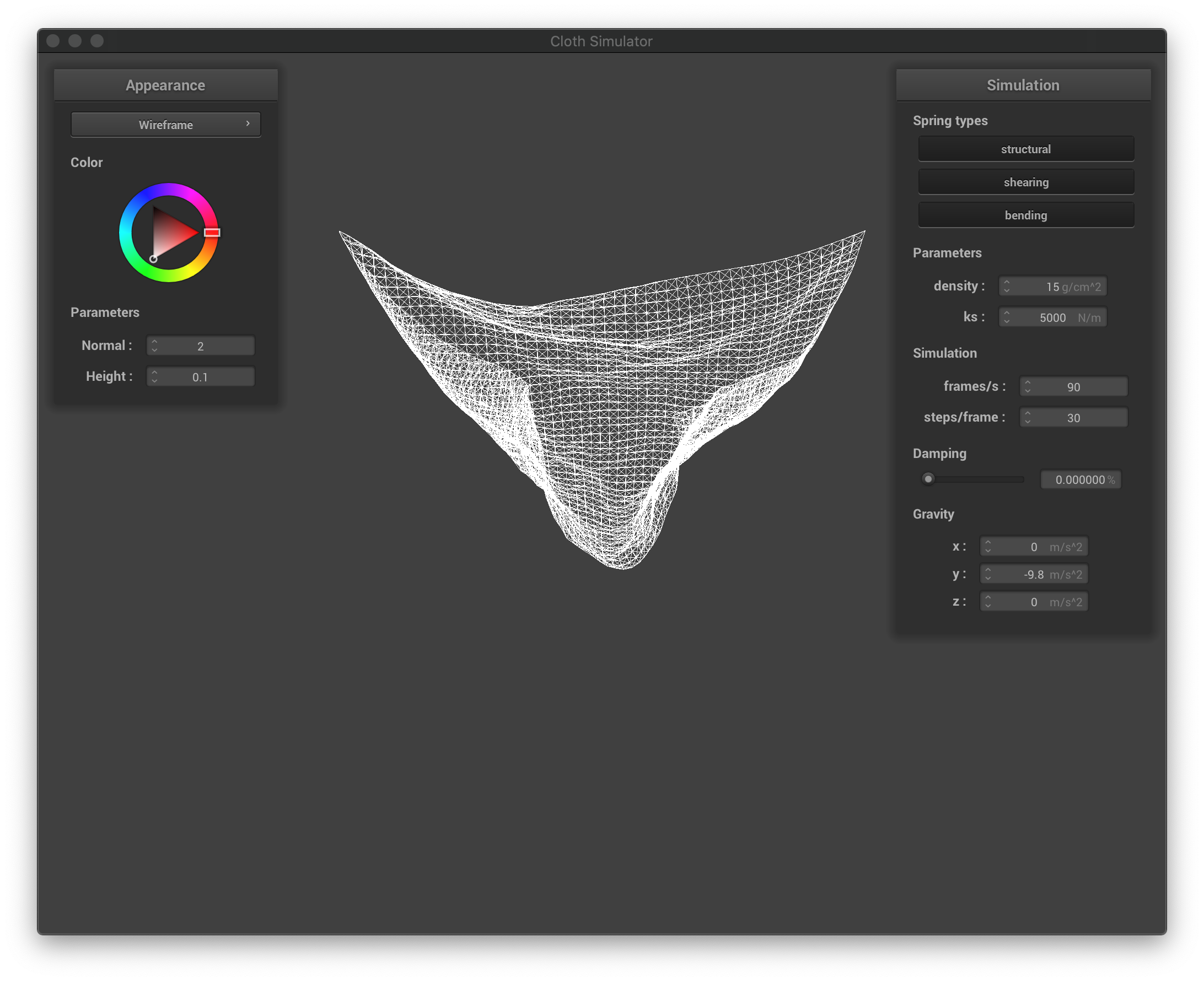 The wireframe with zero damping factor. The cloth swings to the other side.
|
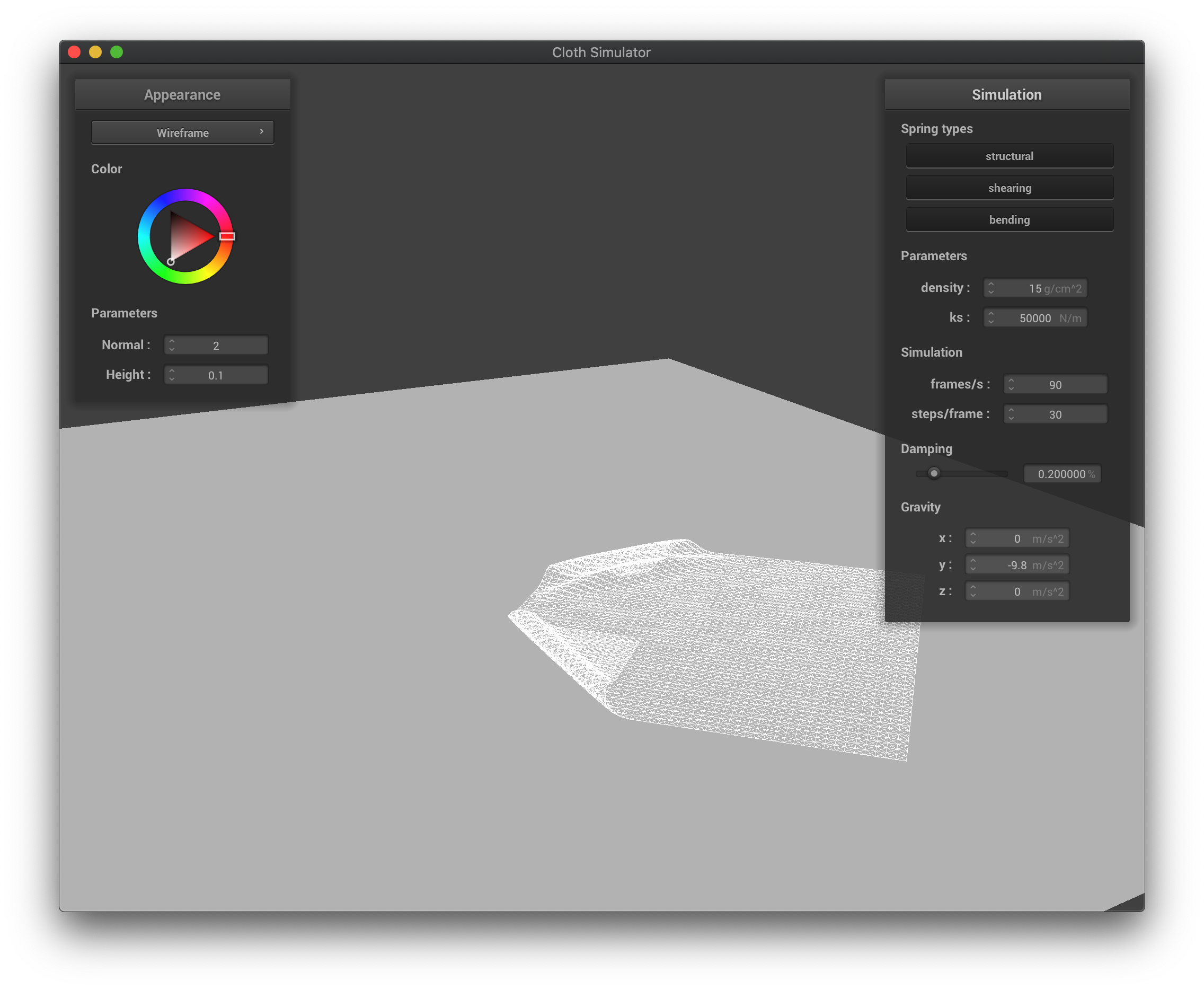
 The wireframe in its final state for scene/pinned4.json.
|
Part III: Handling collisions with other objects
To handle collisions with other objects, we first loop through every point mass looking for collisions with every object. If the object is a sphere,
we check if the mass is inside or on the sphere. Specifically, we check if the following condition is meet:
(pm.position.x-origin.x)^2 + (pm.position.y-origin.y)^2 + (pm.position.z-origin.z)^2 <= radius^2
If so, we calculate the tangent point, correction vector, and update the position as follows:
tangent_pt = origin + radius*(pm.position-origin).unit()
correction = tangent_pt - pm.last_position
pm.position = (1-friction)*correction + pm.last_position
If the object is a plane, we check if the following condition:
dot(pm.position-point, normal) <= 0
If so, we calculate the tangent point, correction vector, and update the position as follows:
tangent_pt = pm.position - pt1_inter*normal
correction = tangent_pt + normal*SURFACE_OFFSET - pm.last_position
pm.position = (1-friction)*correction + pm.last_position
The following pictures show the result:
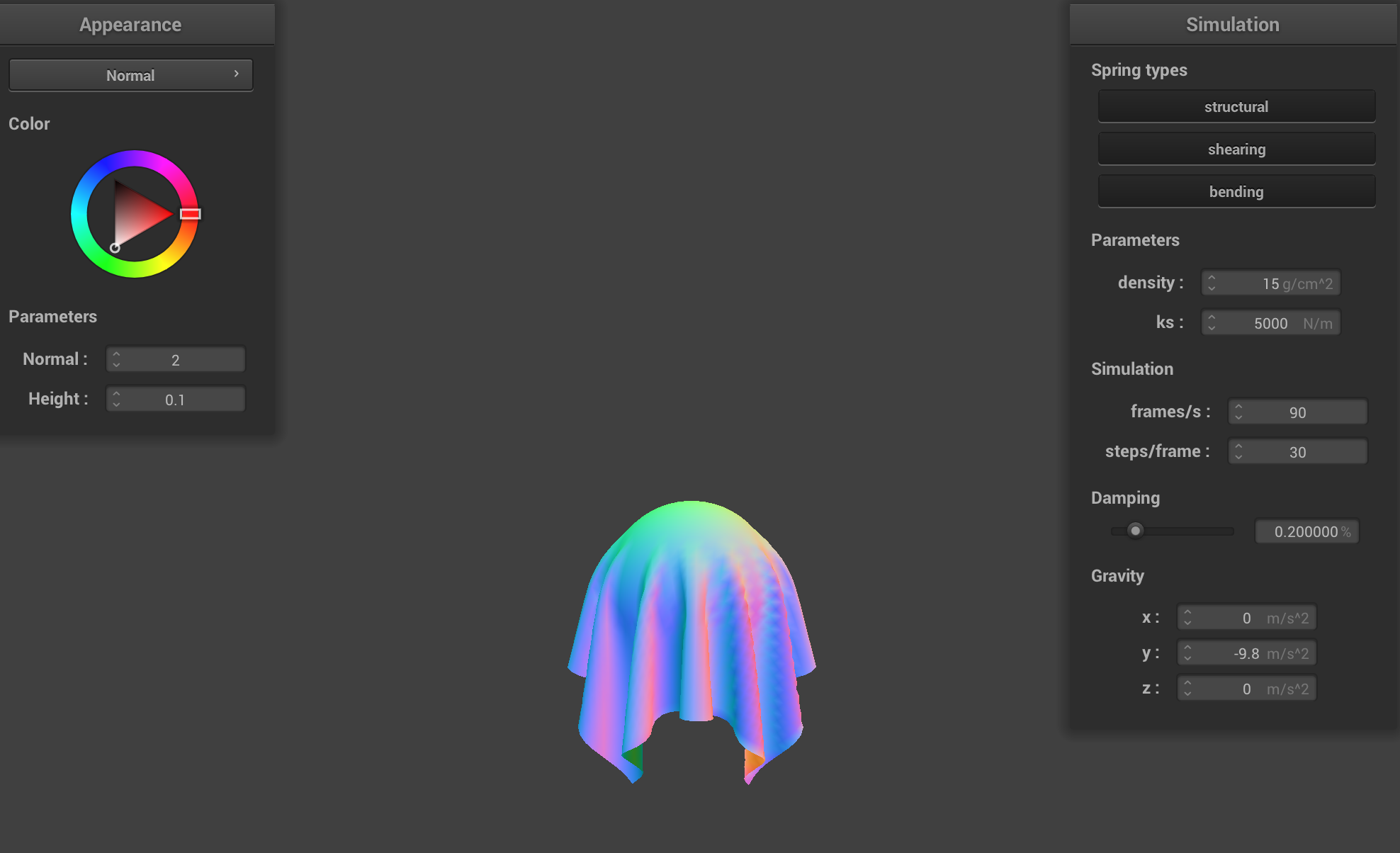 scene/sphere.json in its final resting state on the sphere using the default ks = 5000.
|
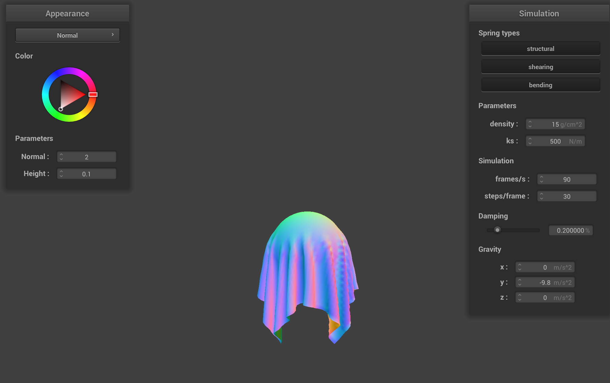 scene/sphere.json in its final resting state on the sphere using ks = 500.
|
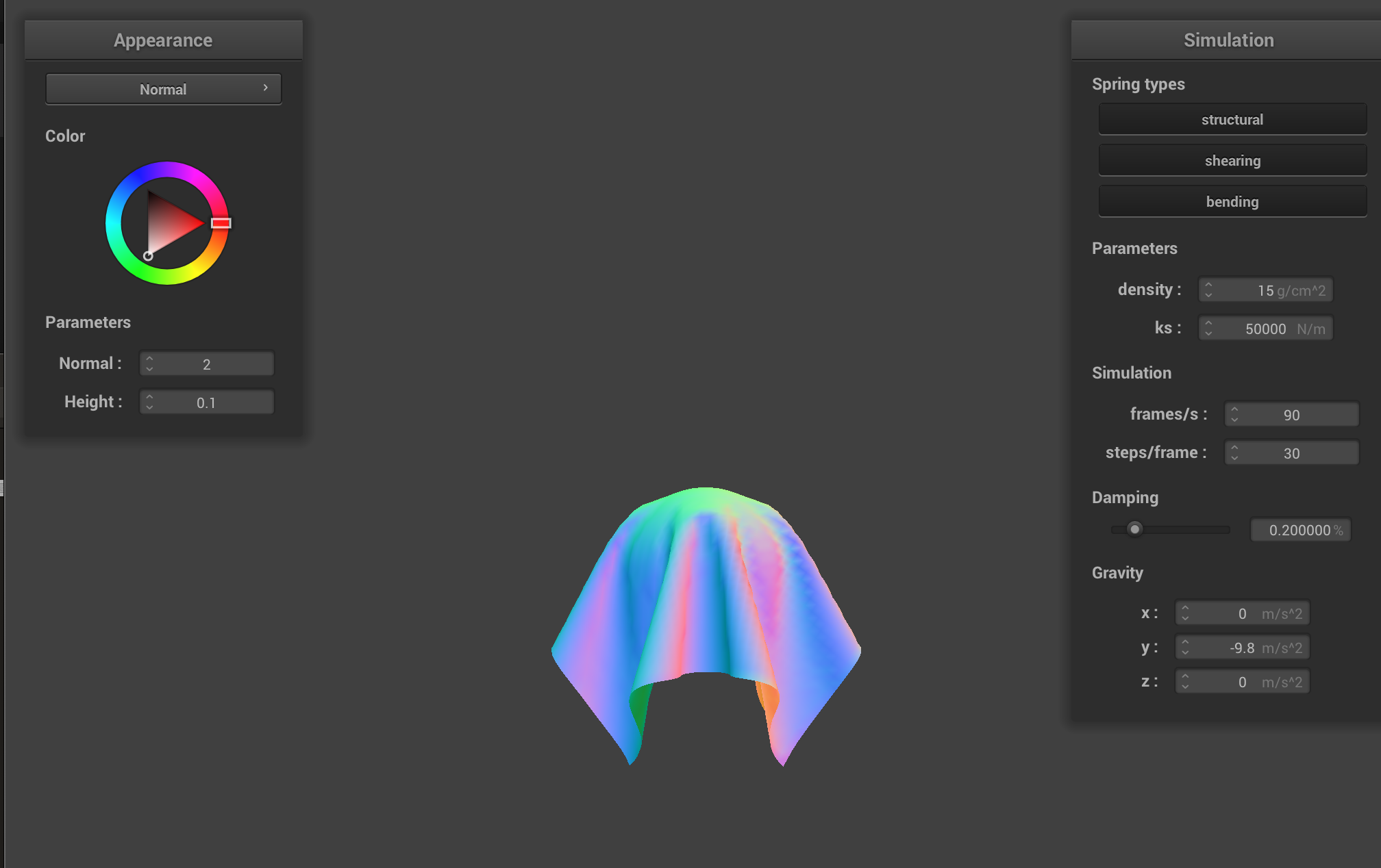 scene/sphere.json in its final resting state on the sphere using ks = 50000.
|
The difference between the above images is that, with ks being large, the cloth looks really stiff. With ks being small, the cloth is soft.
 A screenshot of shaded cloth lying peacefully at rest on the plane.
|
Part IV: Handling self-collisions
To handle self collisions, we first need to accelerate the process of looking for collisions. We need to take a point mass’s position and hash it to the 3D box volume and return a unique hash value. We achieve this goal by computing (w, h, t) according to the width, num_width_points, and num_height_points. Then, we simply return the floor of the pos (x, y, z) divided by (w, h, t) respectively as our hash.
Now, we move on to build a spatial map. For all point masses, we calculate their respective position hash, and check if there exists a vector of point masses with the same hash, and put the point mass into that vector.
Then, we can handle the self collision function. We find if there exists a point mass that is within the 3D box volume and too close to the point mass we passed in. If so, we compute a correction vector that sets the passed in point mass 2 * thickness away from the collided point mass. We then average the result and apply to the passed in point mass.
Finally, we enable self collision by calling build_spatial_map() in simulate() and self_collide() on each point mass. Now, we can demonstrate the process of a cloth falling down on itself:
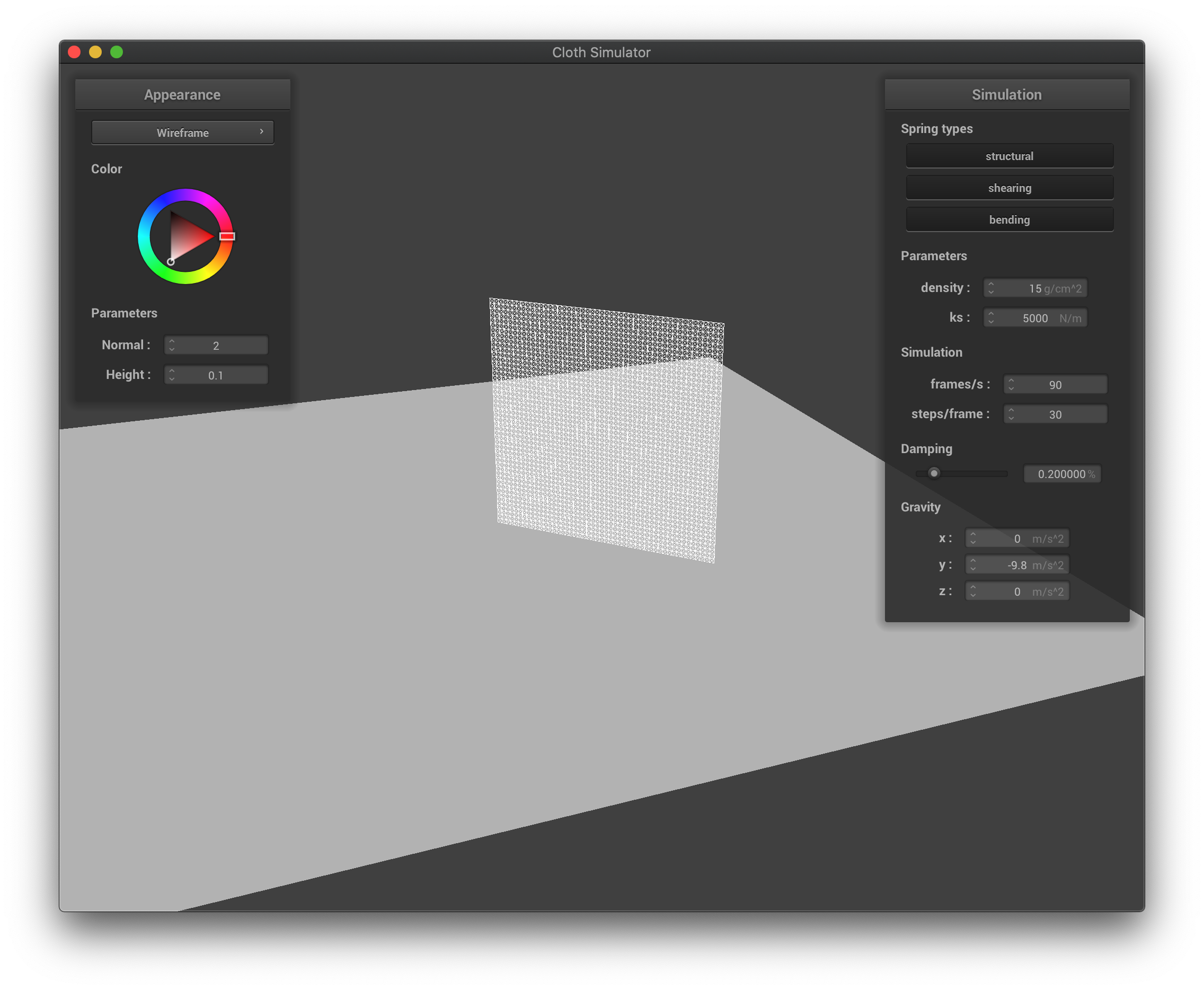 The wireframe before falling down.
|
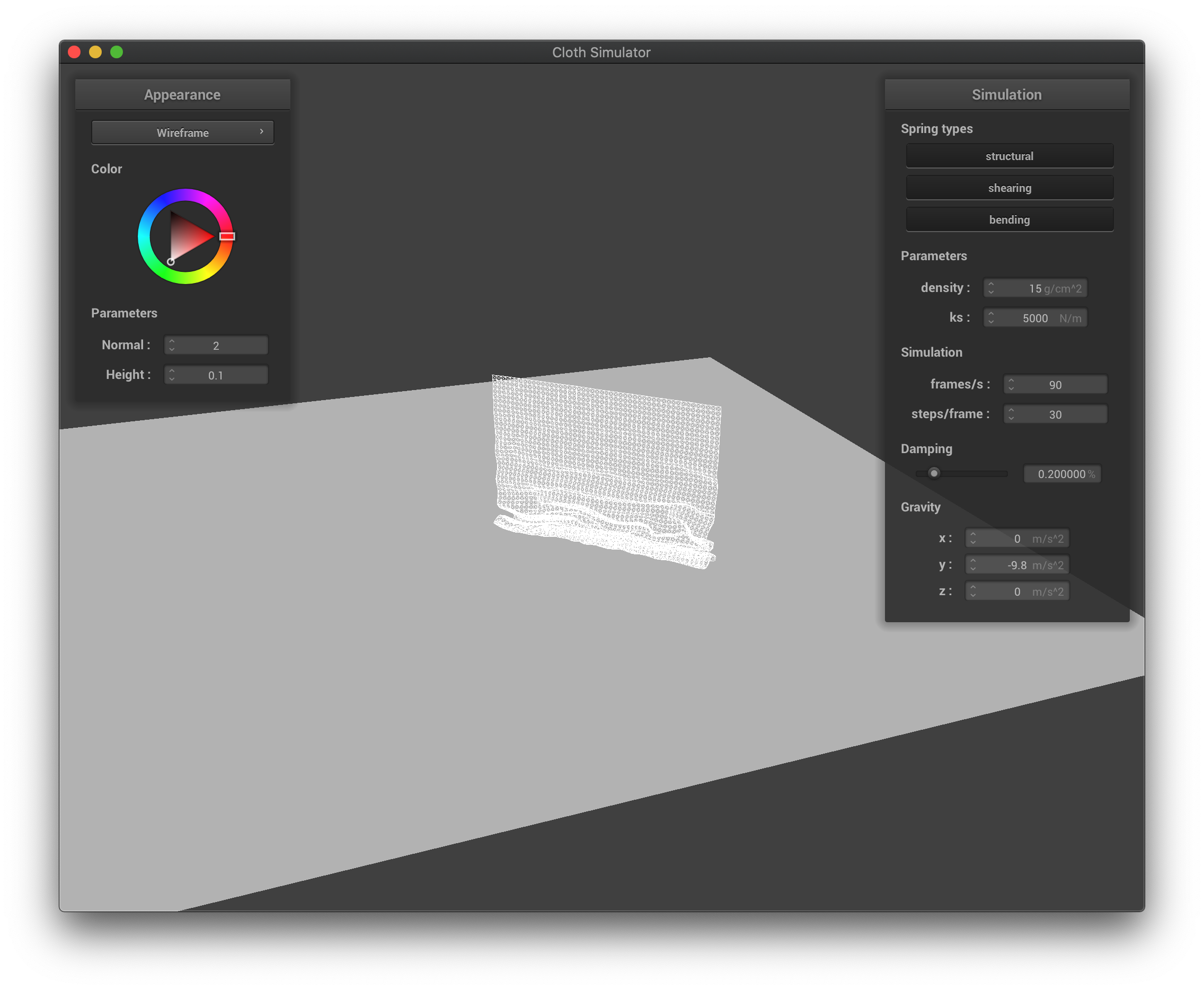 The wireframe at first collisions when falling down.
|
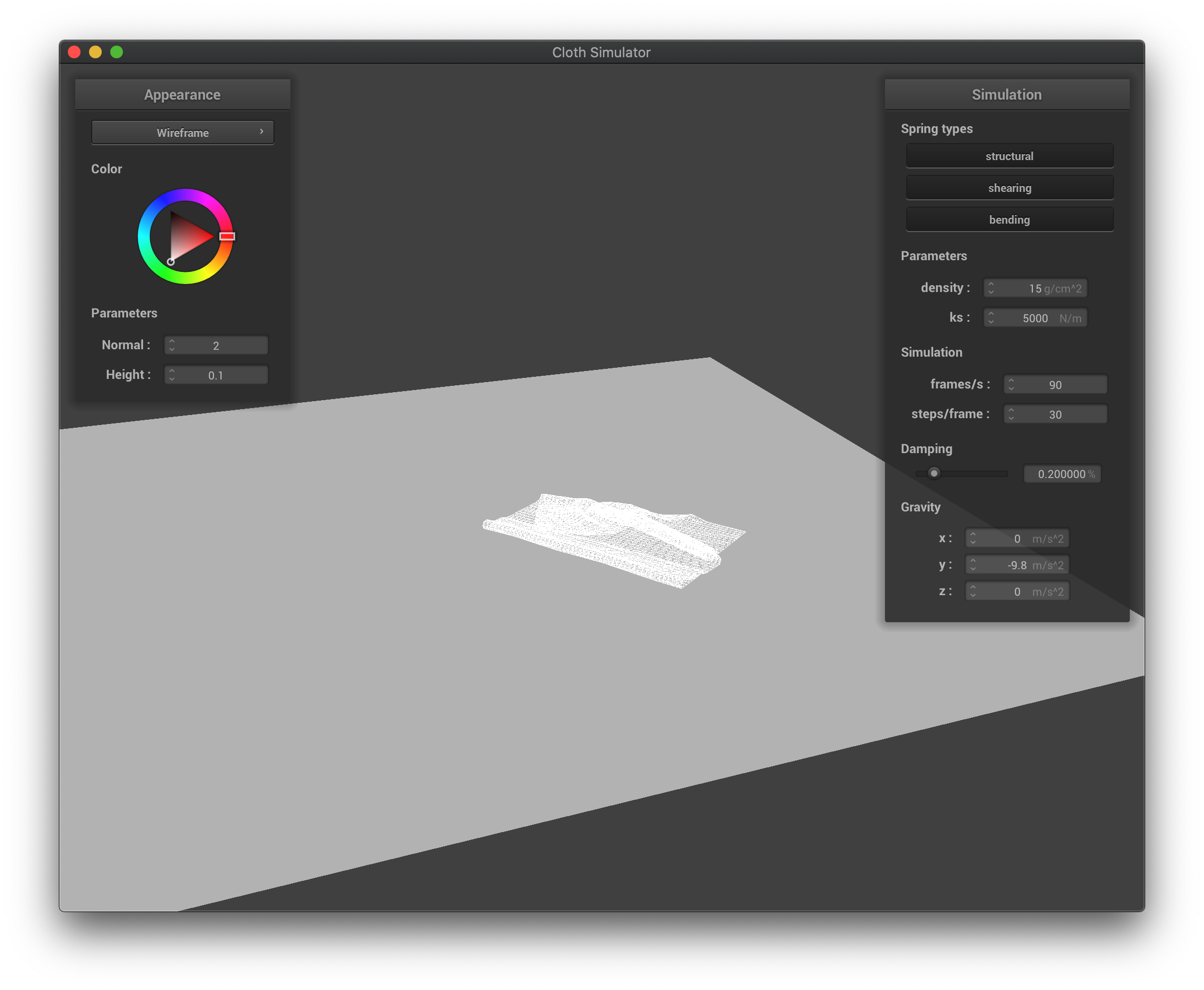 The wireframe at its final state after falling down.
|
If the density is higher, the cloth falls into a more compact shape with a lot of folds, and while falling, there are also more wrinkles on the cloth. The cloth bounces off less from itself as collisions happen. If the density is lower, the cloth falls into a more spread-out shape, where there could be few folds only, and while falling, there are also less wrinkles on the cloth. The cloth bounces off itself more easily as collisions happen.
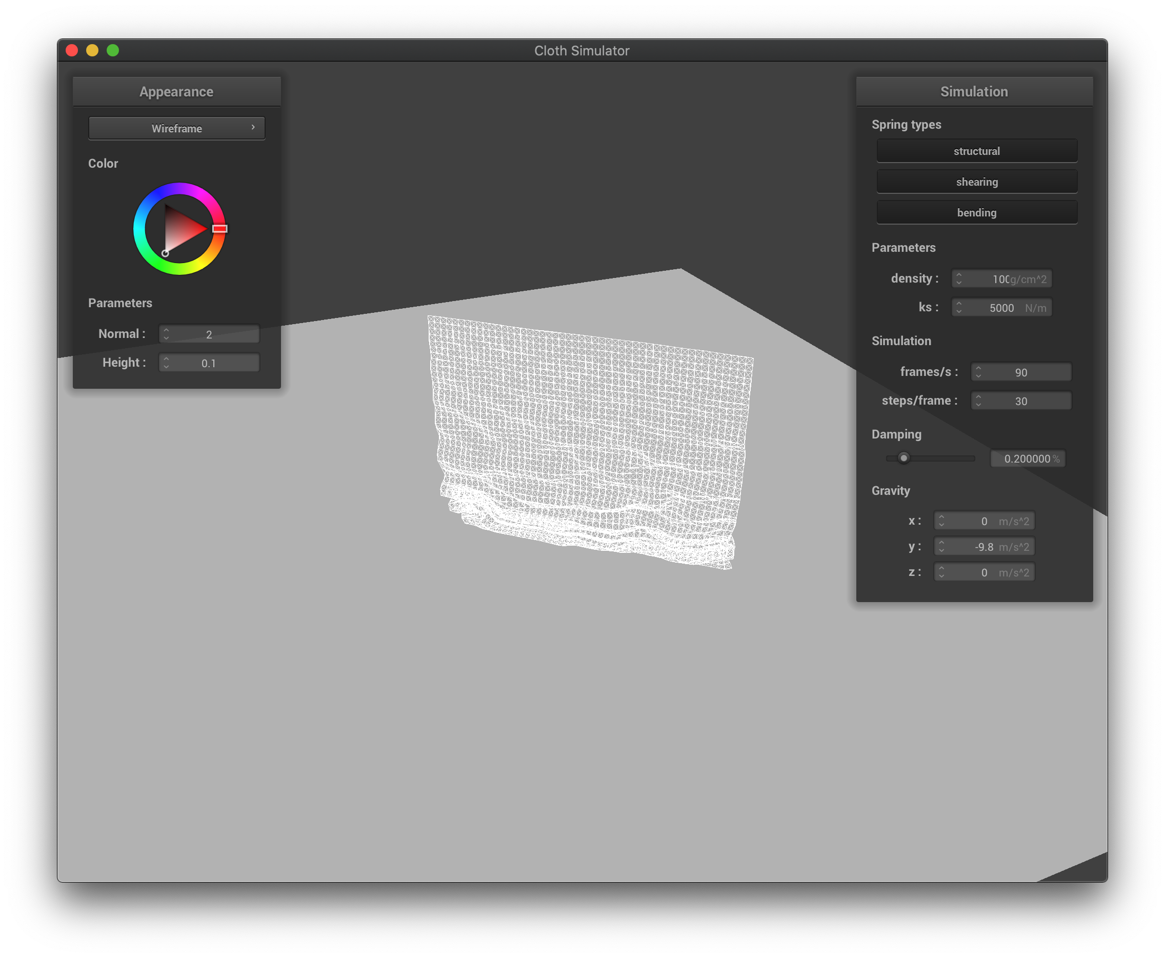 The wireframe with high density at its first collisions when falling down.
|
 The wireframe with high density in the middle of falling down.
|
 The wireframe with high density at its final state after falling down.
|
 The wireframe with low density at its first collisions when falling down.
|
 The wireframe with low density in the middle of falling down.
|
 The wireframe with low density at its final state after falling down.
|
If the spring constant is higher, the cloth falls into a more stretched-out shape, as there will be more forces exerted during compression, and the cloth is maintaining a flatter shape for the part that is yet to collide with itself. If the spring constant ls lower, the cloth now supports itself less, and falls into a more compact shape due to not enough force exerted during compression to spread itself out, and the cloth is full of wrinkle when falling down.
 The wireframe with high spring constant at its first collisions when falling down.
|
 The wireframe with high spring constant in the middle of falling down.
|
 The wireframe with high spring constant at its final state after falling down.
|
 The wireframe with low spring constant at its first collisions when falling down.
|
 The wireframe with low spring constant in the middle of falling down.
|
 The wireframe with low spring constant at its final state after falling down.
|
Part V: Environment-mapped Reflections
Shader program runs on GPU. It effectively gives triangle meshes shape and color. Vertex shaders alter the (final) position, normal of vertex, while fragment shaders take in the properties of a vertex from vertex shaders anf output the color.
In Blinn-Phong shading, we break lighting down to three different parts: ambient lighting, diffuse reflection, and specular highlights. This enables us to present different lighting effects using different calculation methods/models and combine them together. We simply compute the elements within each method with the given parameters and plug them into the formula to yield the final result. We choose p = 100, k_a = 0.1, k_s = 0.6, k_d = 1.0 as the coefficients.
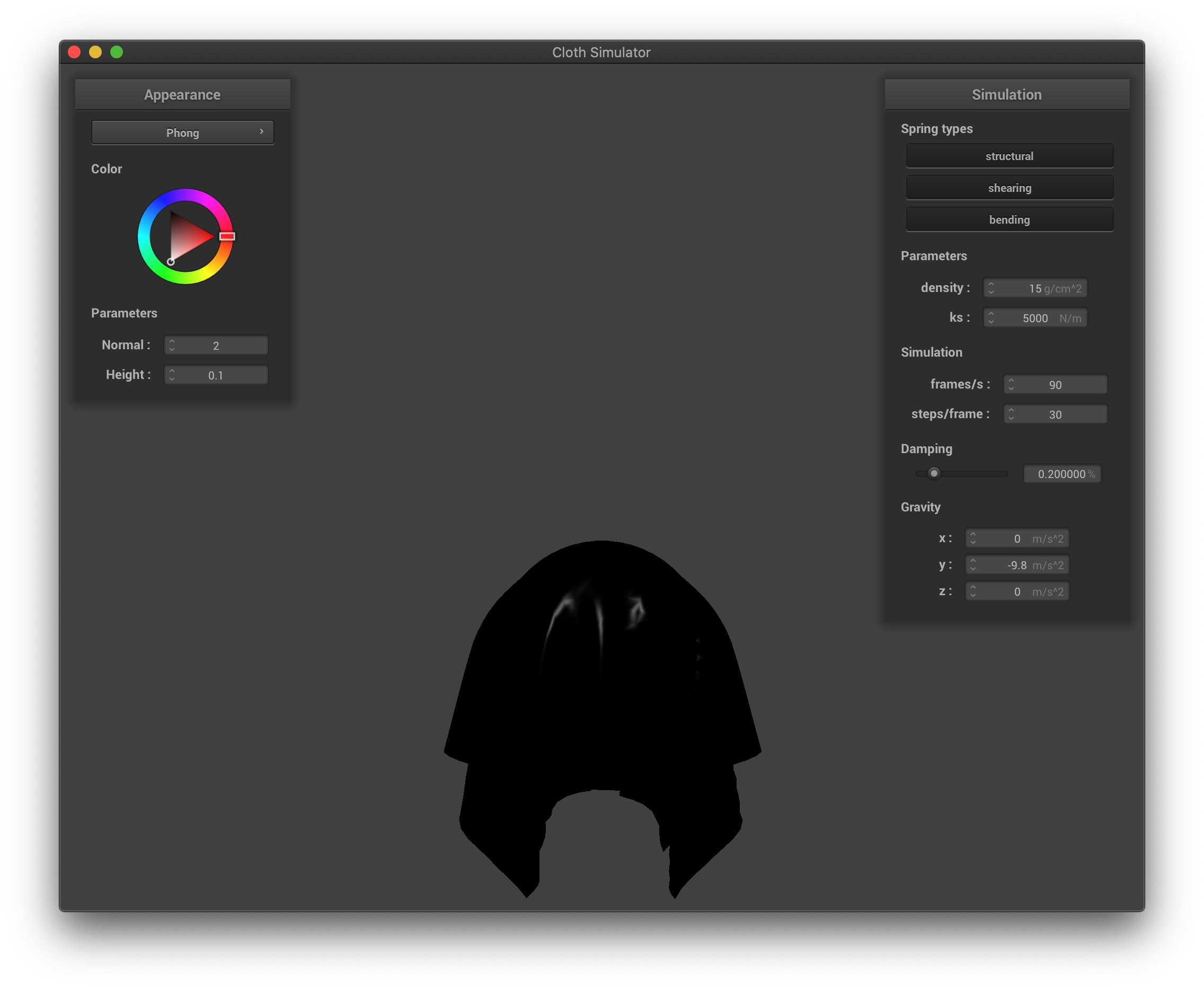 The Blinn-Phong shading only with specular lighting.
|
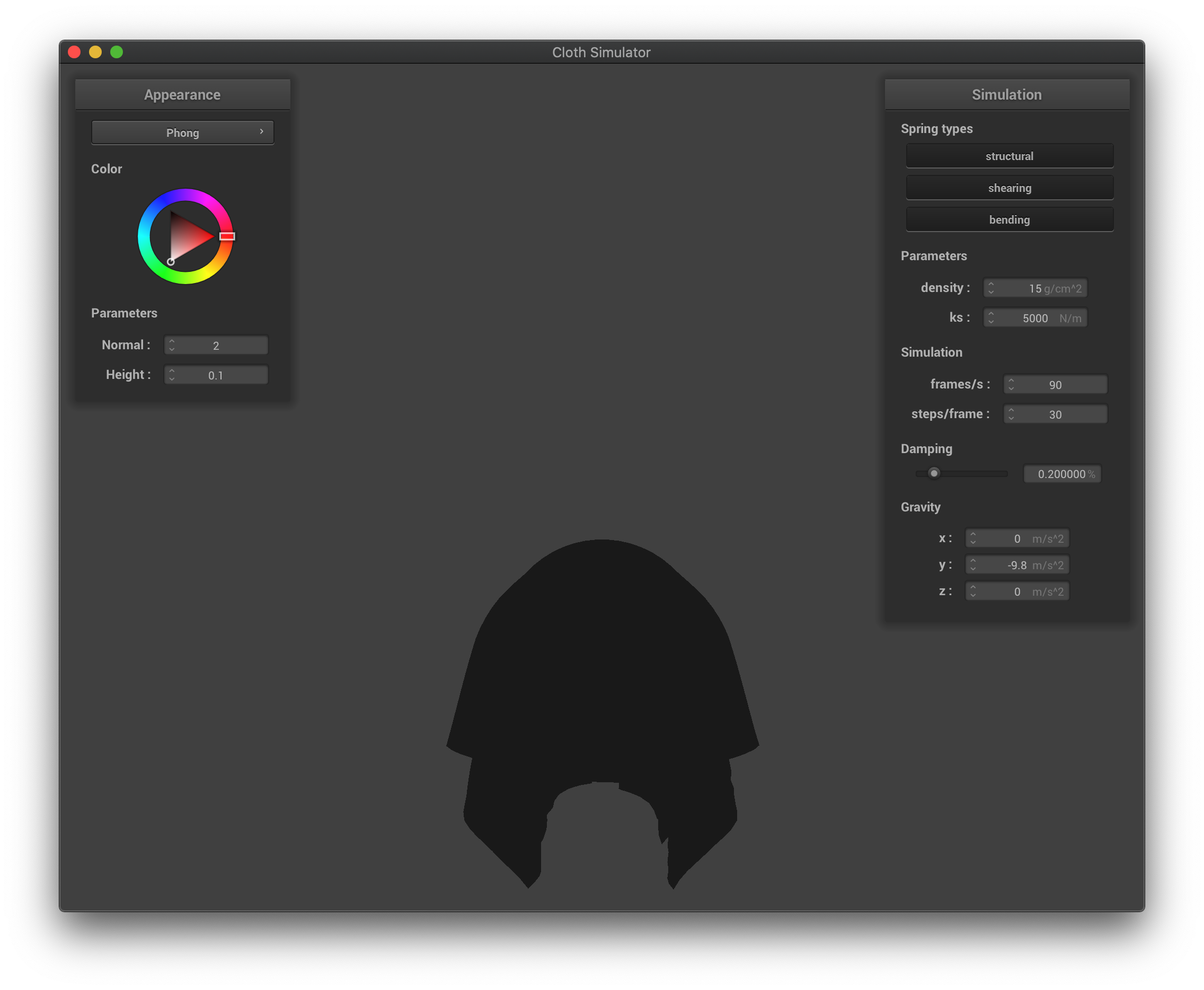
 The Blinn-Phong shading only with diffuse reflection.
|
 The Blinn-Phong shading only with ambient lighting.
|
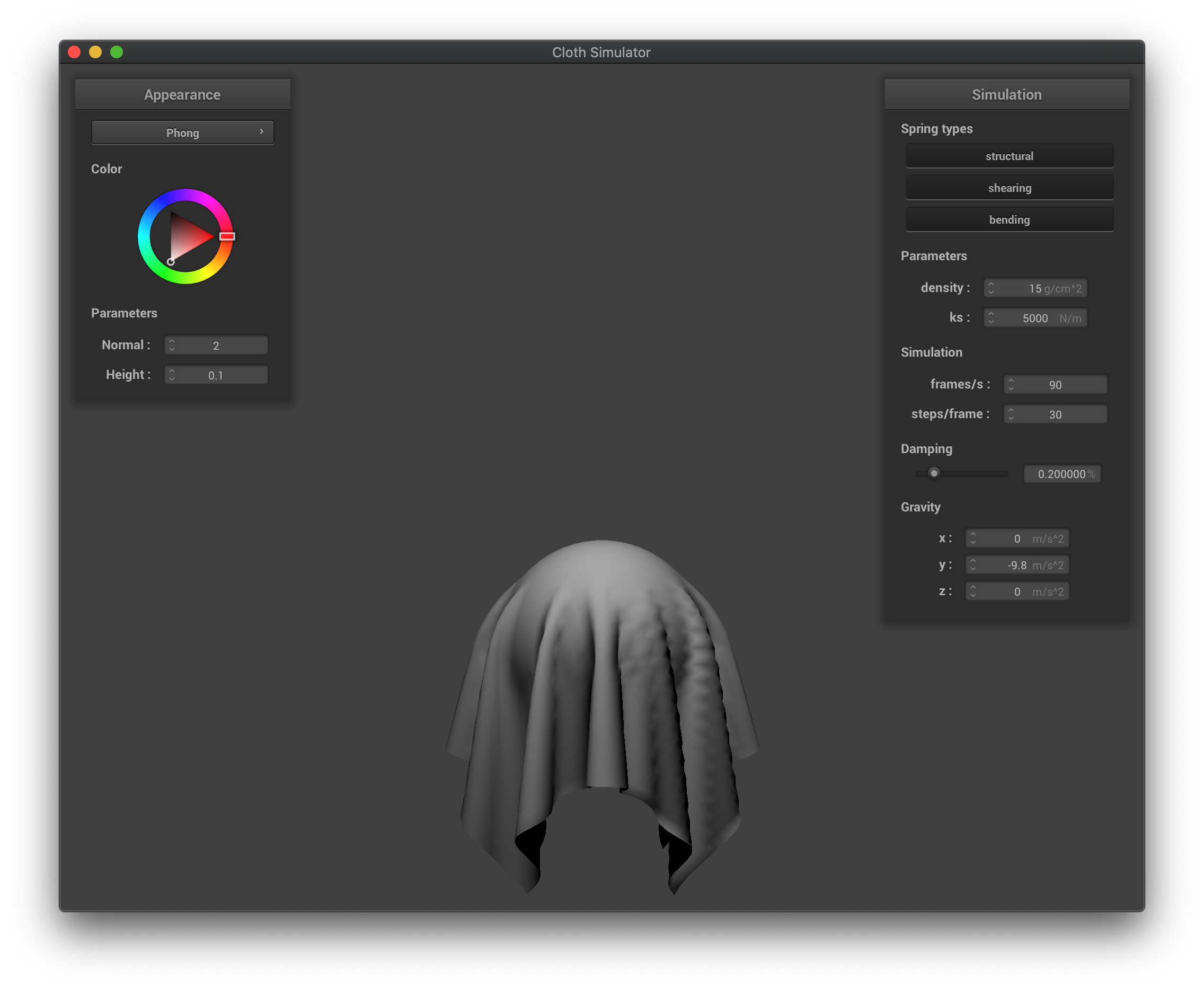
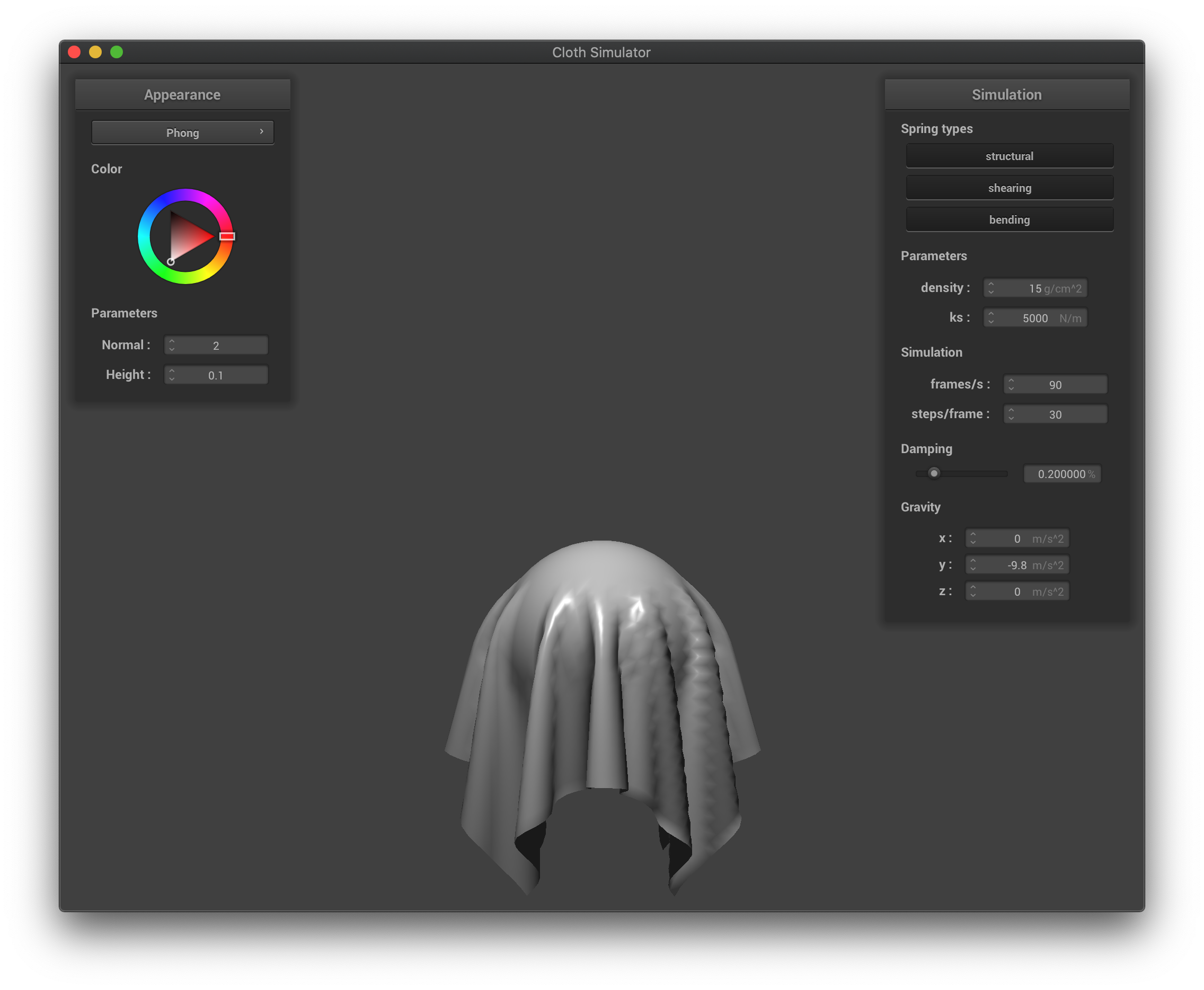 The Blinn-Phong shading overall effect.
|
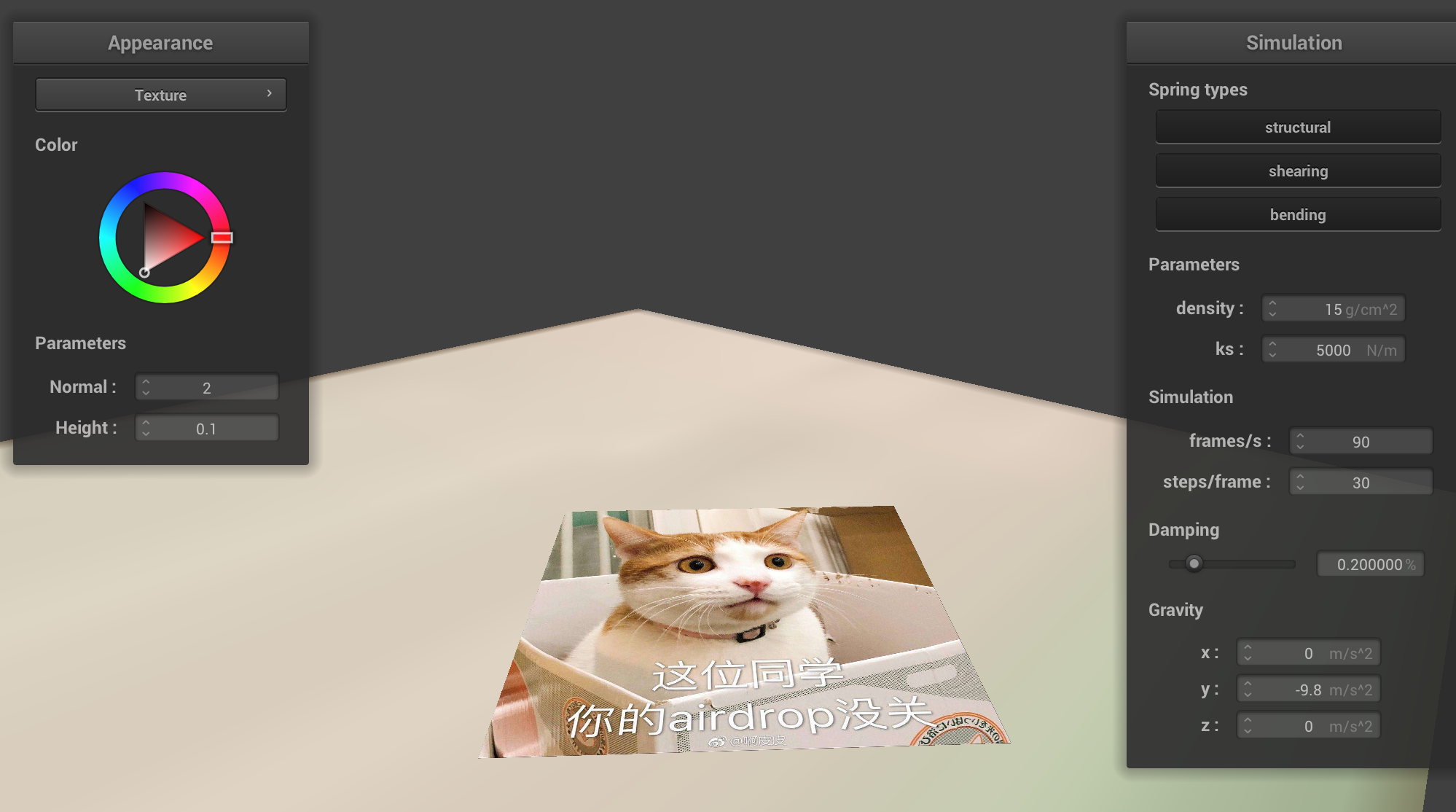
For texture mapping, we simply call the texture() function in GLSL to map a texture on the objects.
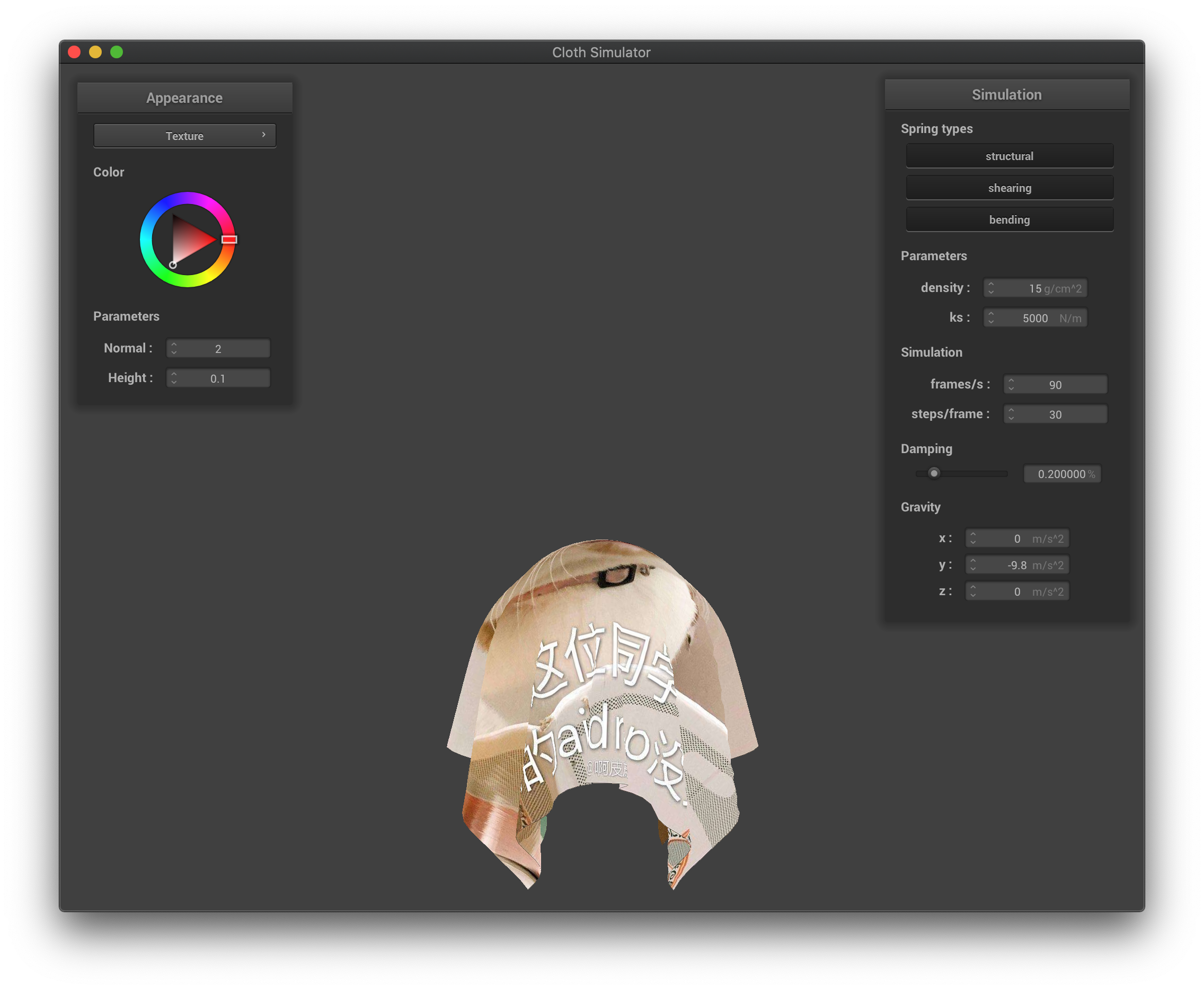 The texture mapping with custom texture.
|
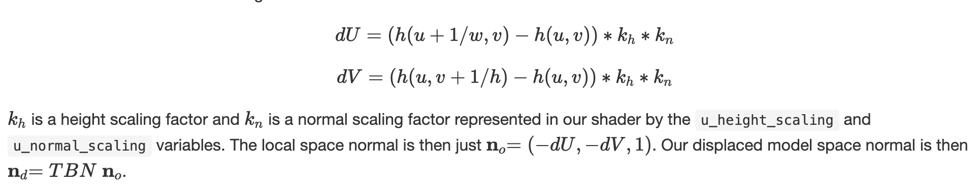
For bump mapping, we transform the normal vector by first computing local space normal no. Equations are shown below:
 no equation.
|
The final normal is nd which equation is show above. TBN matrix is [t b n] where b = n x t. After computing the new normal nd, we copy the phong shading code then replace the old normal with new normal.
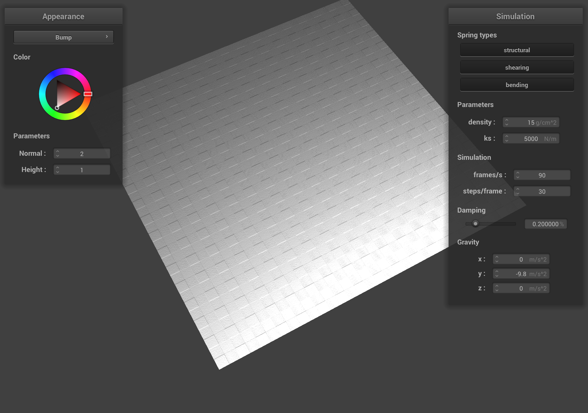 A screenshot of bump mapping on the cloth.
|
 A screenshot of bump mapping on the sphere.
|
For displacement shading, compare to bump shading, we only change the vertex shaders. In particular, we add in_normal * h(in_uv) * u_height_scaling to position, normal, and tangent.
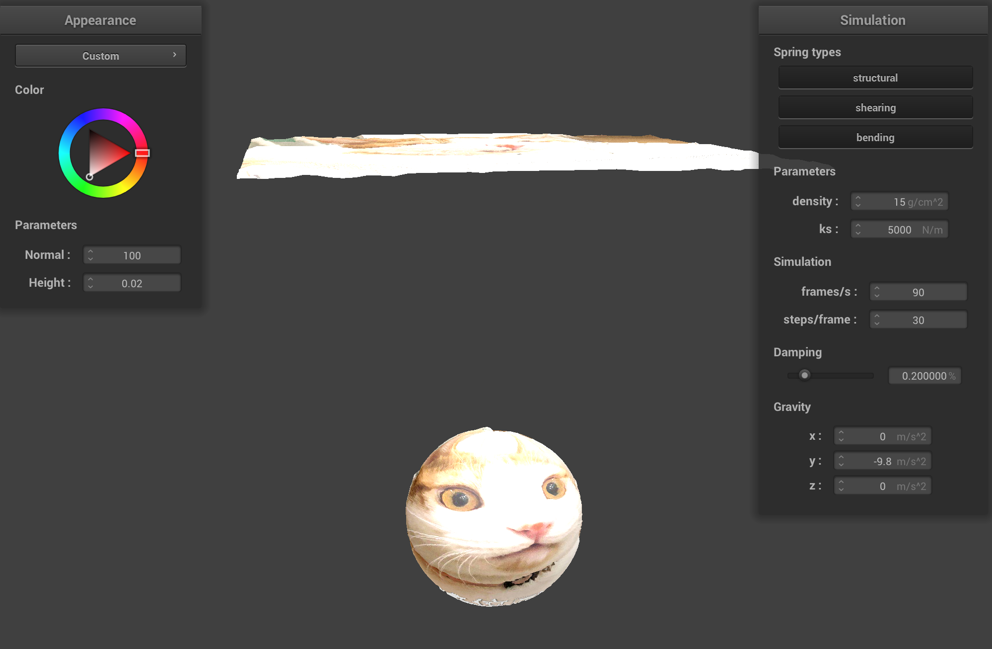
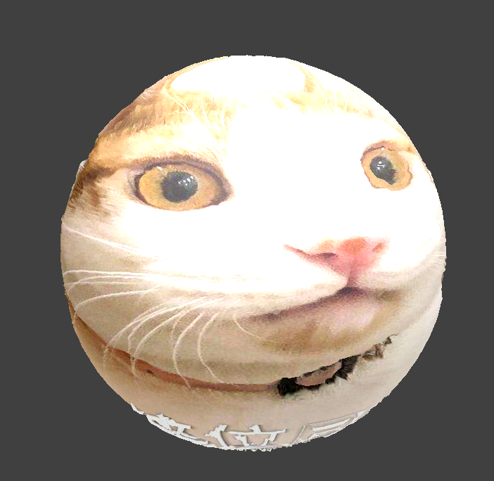
 A screenshot of displacement mapping on the sphere.
|
The difference in the resulting shading is that displacement shading has uneven surface but bump shading has smooth surface.
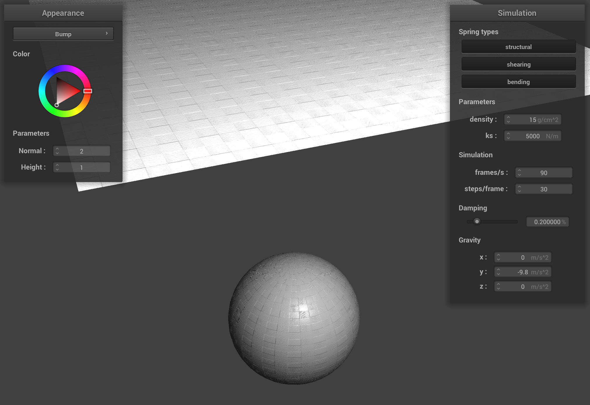
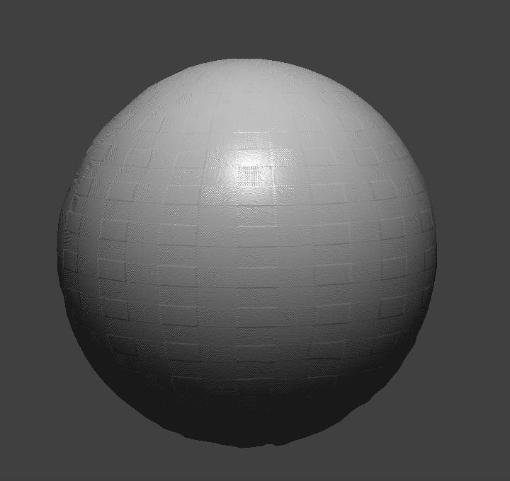
 Bump shading with -o 16 -a 16.
|
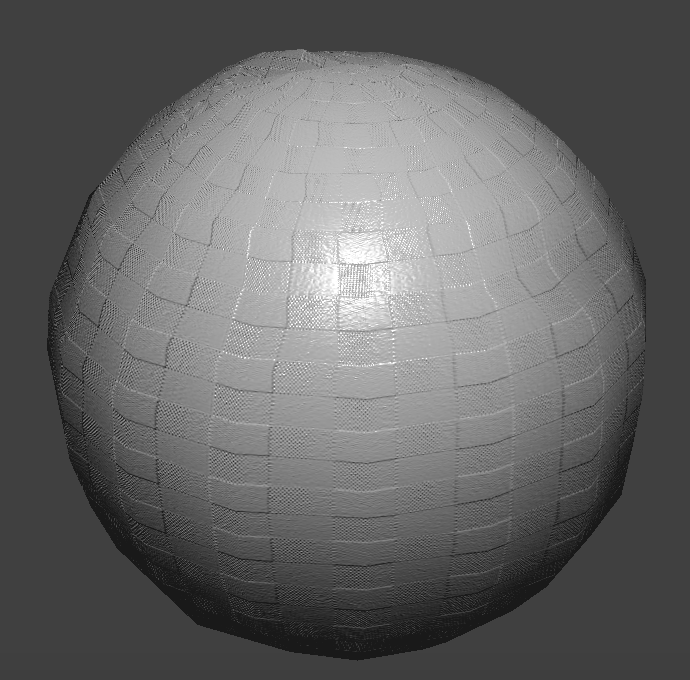 Displacement shading with -o 16 -a 16.
|
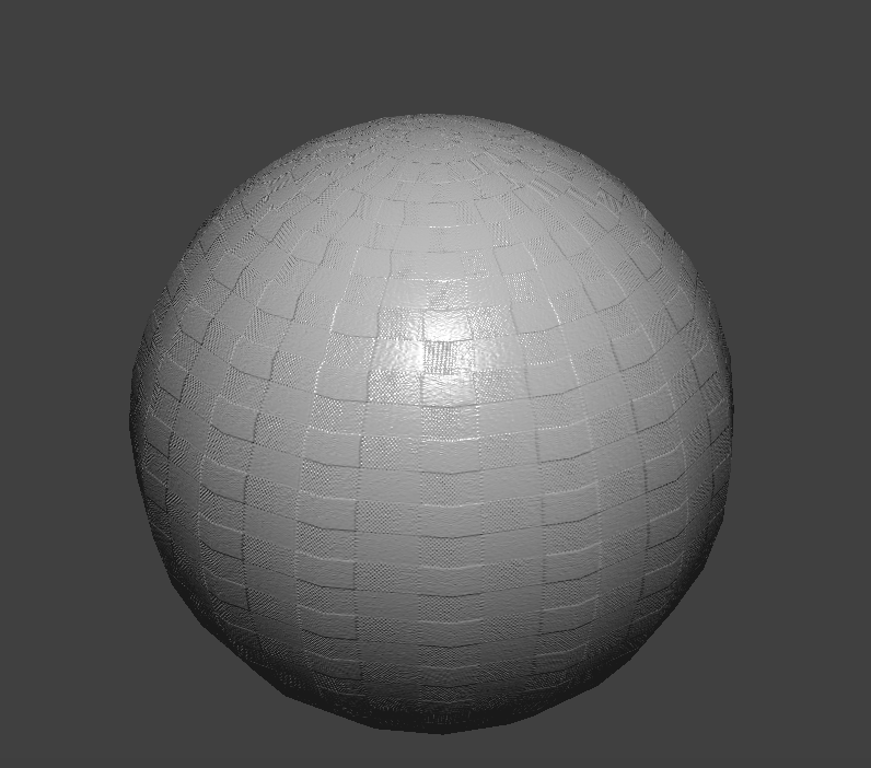
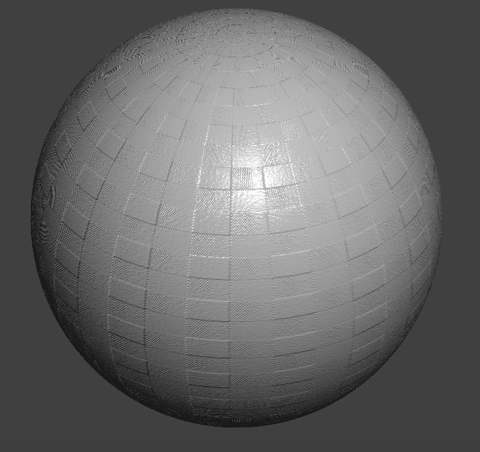 Bump shading with -o 128 -a 128.
|
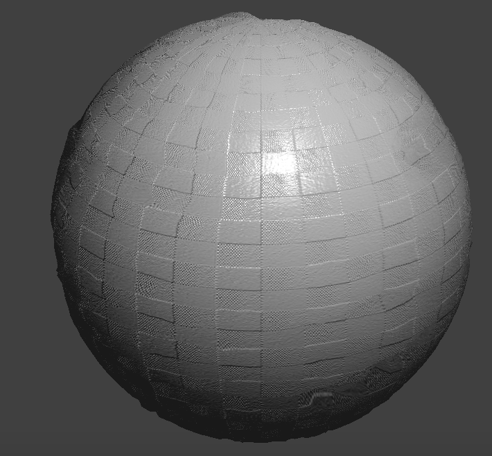 Displacement shading with -o 128 -a 128.
|
With different sphere mesh's coarseness as shown above, the two shading behaves differently. With -o 16 -a 16, the bump shading sphere is not smooth and displacement shading has large bumps.
With -o 128 -a 128, the bump shading sphere is smooth and displacement shading has small bumps.
For mirror reflection, we calculate the vector from the reflection point to the camera and use that combined with the surface normal to compute trace back the ray. We simply call texture() on the trace back ray in the reverse direction to find the output color.
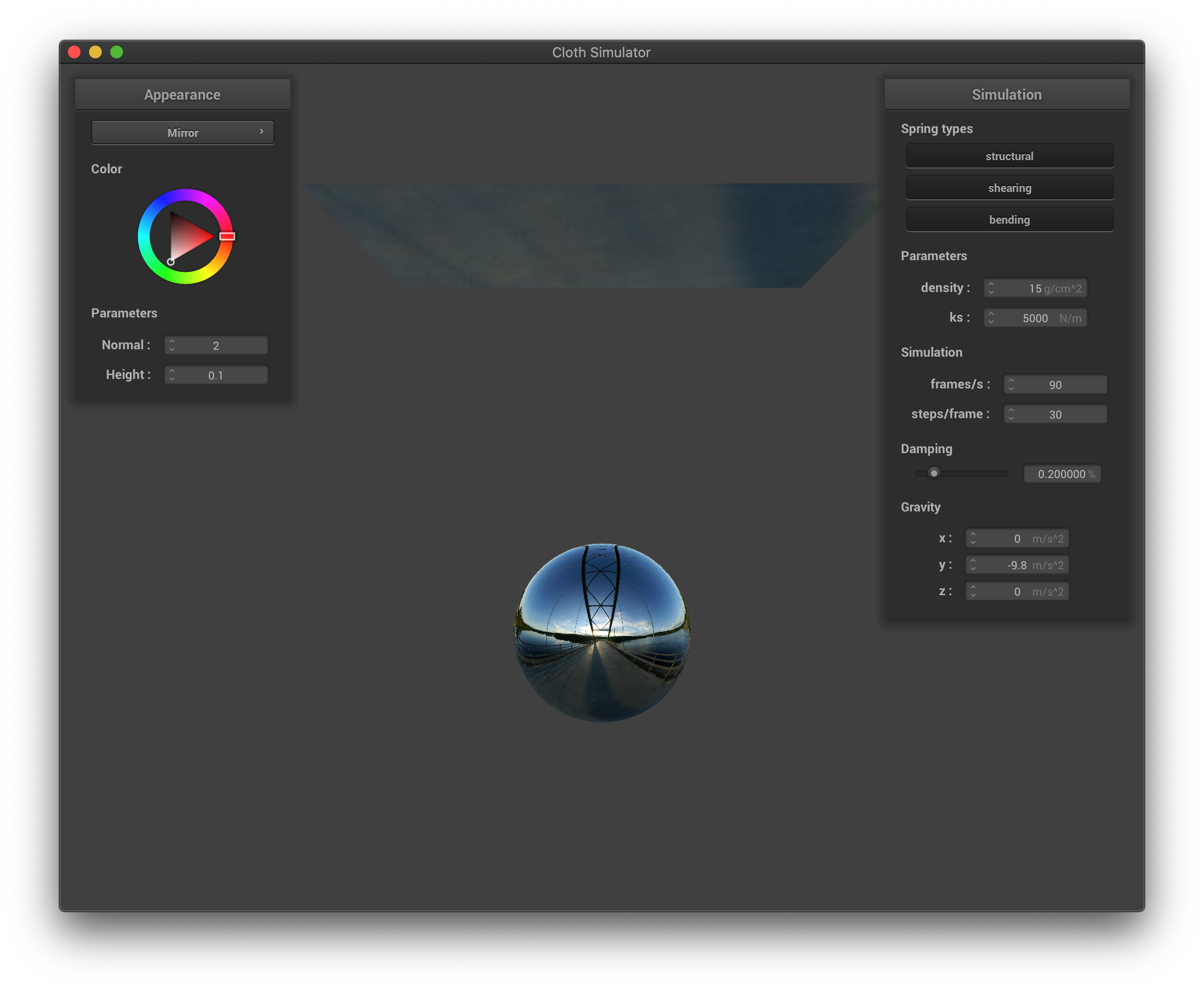 The mirror shading before simulation.
|
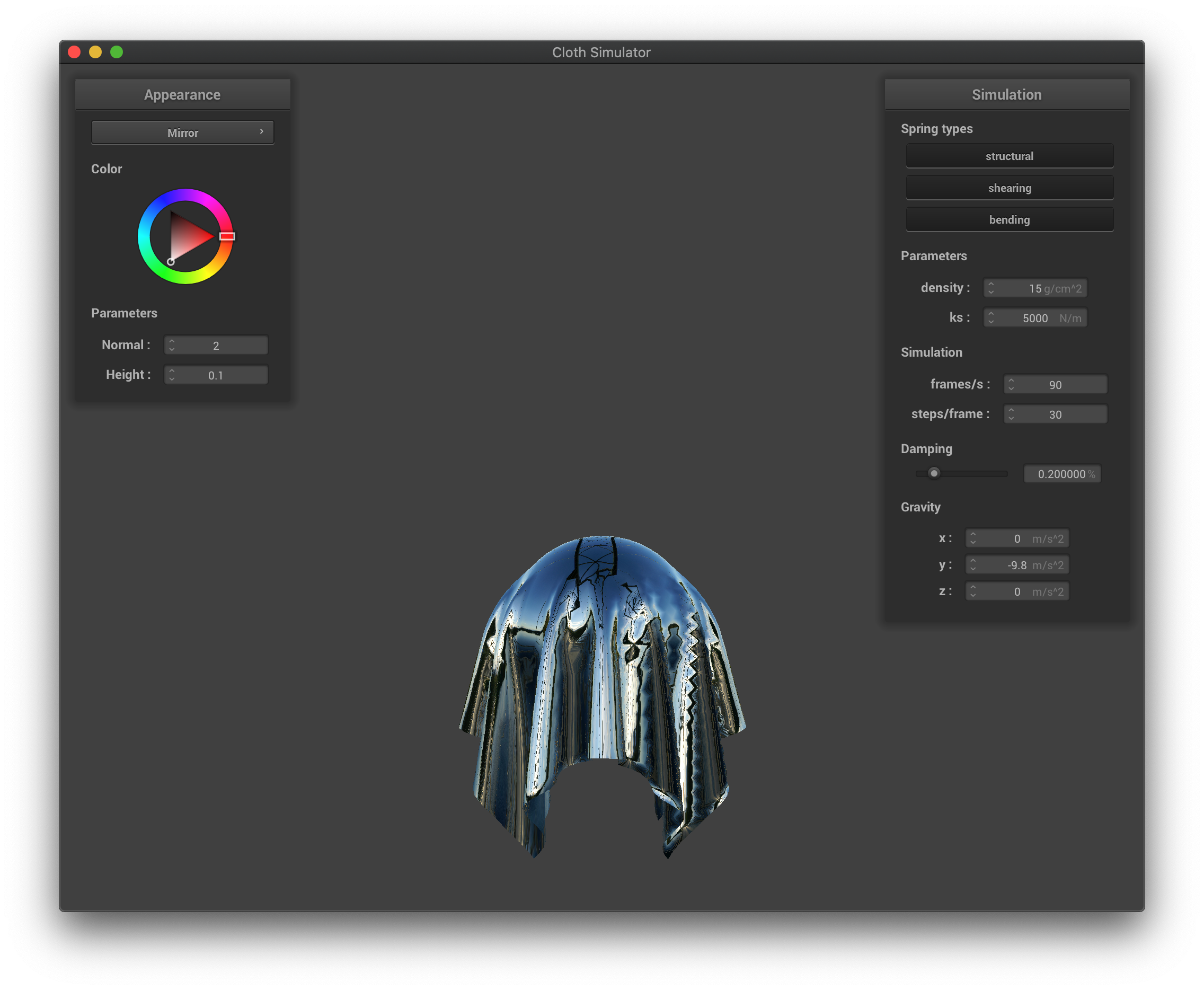 The mirror shading after simulation.
|
Part VI: Extra Credit
For custom shading, we implement displacement diffuse texture giving a silk texture. Specifically, we copy the displacement implementation for vertex shader.
For fragment shader, we take the texture and add a diffuse term. The diffuse term is taken directly from phong shading.
 Custom shading.
|