Our group attempted to render scenes of sky and halos.
We rendered the sky using volume rendering with two different types of atmospheric scattering: Rayleigh and Mie.
We also delved into tone mapping to generate realistic images, and acceleration structure to real time sky rendering.
We further added the feature of rendering halos around the sun from physical computation and color mapping. We managed to provide fast rendering of the sky with different viewing perspectives as well as features of adding halos.
Model
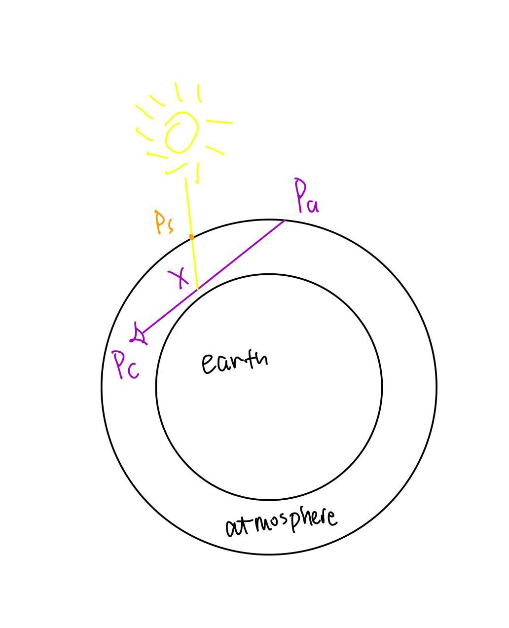
The atmosphere model we'll be using in our final project is defined as two concentric spheres.
The center is always at (0, 0, 0).
The inner sphere represents the Earth. The Earth's radius is defined to be 6360 km.
The outer sphere represents the atmosphere. The atmosphere radius is defined to be 6420 km.
We define the sun as being infinitely far away from us, so the sun light reaching the Earth is modeled as parraleled light.
The sun lies on the yz plane.
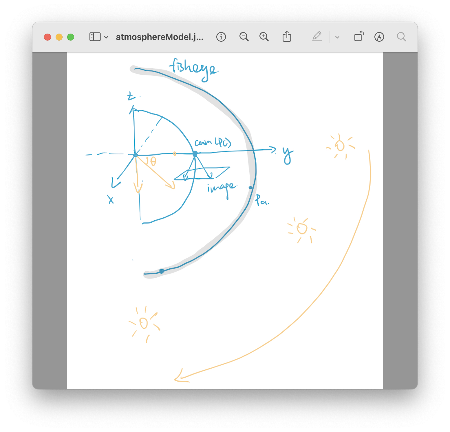
It's direction is specified by angel $\theta$, which is the angle between the sun and y axis.
We are able to represent two kinds of images with this model.
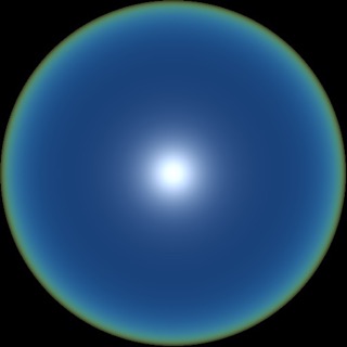
Fisheye
Fisheye images are rendered by specifying a camera location (Pc) and looking up from the camera at the sky. The image captures all 360 degree view.
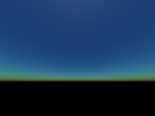
Normal Camera
Normal camera images are rendered by specifying a camera location (Pc) with a FOV. We specify a plane on the z axis for our image,
and calculate the size of the image in world space by using the size of image we want to render and FOV of our camera.
Fisheye Camera
Normal Camera
Below is an illustration of our atmosphere model.
Volume Rendering: Technical Approach
The most central idea to our project is Volume Rendering, as this is how we determine the color of every pixel. We
learned about Volume Render mostly from a series
of online lessons provided by Scratchapixel.
Scattering
The atmosphere is not vacuum. It contains small air particles and aerosols, and they caused scattering effects. We
will be focusing on 2 kinds of scattering:
Rayleigh scattering: scattering by small particles such as air particles
Mie Scattering: scattering by aerosols such as dust. These molecules are generally bigger.
While the sunlight is usually not directly toward our eyes, we still can see light on the sky, and this is because
sun light is being deflected and scattered by particles
the light encountered. These scattering effects dominated the color and intensity of light that the camera ray
received.
Out-scattering is the main reason why in the atmosphere, as light travels, it diminishes. The amount of light that
can pass throught the atmosphere is governed by Beer-Lamber Law, and the transmittence of that in that medium
is \(T = e^{-distance*\sigma}\), where \(\sigma\) is the scattering coefficient of the medium. The equations for
Rayleigh and Mie scattering can tell us this coefficient.
For Rayleigh scattering, $$\beta(h) = \frac{8\pi^3(n^2-1)^2}{3N\lambda^4}e^{-\frac{h}{H_R}}$$
\(h\) is the height
of which we are calculating the scattering coefficient.
For Mie scattering, $$\beta(h) = \beta(0)e^{-\frac{h}{H_M}}$$
\(\beta(0)\) is the Mie scattering coefficient at sea
level. \(h\) is the height of which we are calculating the scattering coefficient.
Therefore, both scattering coefficients vavaries with elevation.
Rendering the Volume
For every pixel on the screen, we shoot a ray from the pixel, and integrate along this camera ray to obtain the
final color of the pixel. We will integrate along the purple ray to obtain the final pixel of the source pixel of the purple
ray. The outer circle is the atmosphere, and the inner circle is the earth. \(P_c\) is the position of the
camera,
\(P_a\) is where our camera ray hits the edge of the atmosphere, and \(P_s\) is where the sunlight hits the
atmosphere.
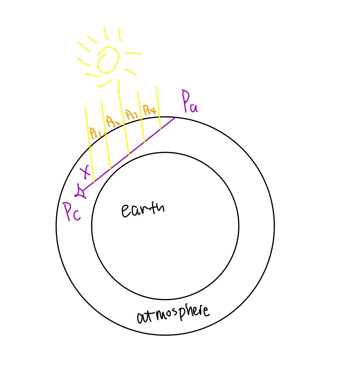
However, since the sun is very far away, sunlight that falls on the earth can roughly be seen as parallel light.
Therefore, our full model looks like this: \(P_{si}\) are where the parallel sunlights hits the atmosphere.
Therefore, at each segment of the camera ray, we have different lights fall on it, because:
Each segment will be occluded by previous segments;
The amount of sunlight received by each segment is also different, as the distance that sunlight need to travel
within the atmosphere in order to hit that segment of the camera Ray
is different.
Therefore, to integrate along the camera ray, for each segment on
the camera ray, we will have to calculate, how much light from the light source falls onto it. This is done by
another integration (so we will also be integrating on the yellow lines
in the diagram above to calculate the amount of light that reaches the intersection of yellow and purple lines). You
might wondering why do we need to integrate along the yellow lines to
obtain the amount of sunlight that reaches the camera ray, instead of simply calculating the transmittence with Beer
Law and multiply it with intensity? Remember that both Rayleight and Mie scattering coefficients varies with
elevation, and as sunlight travels, the elevation changes,
so the transmittence of light changes as it travels. Therefore, the sunlight that reaches one segment $X$ of the
camera ray can be expressed as: $$L_{sun}(X) = Sun\space Intensity * T(X, P_s) * P(V,L)*\beta.$$ $P(V,L)$ is the
phase function for scattering, and it tells us about how much light is scattered for a particular viewing direction.
It's givien by the type of scattering. We will do the integration at the end to combine the two integrals.
After obtaining the amount of light at each segment, we can sum them up to obtain the final color, taking into
consideration that to eventually reach the camera,
the camera ray will also travel through the atmosphere, and scattering will also occur. Therefore, the conceptual
formula is: $$L=\int_{P_c}^{P_a} L_{sun}(X)T(P_c, X)dX,$$ and we
substitute $L_{sun}$ into the integration.
In practice, for each segment, we shoot a ray from the segment, and divide this light source ray into another 8
segments, and sum up their resulted light vector. Then for each segment on the camera ray,
we multiply the sumed light vector with the distance the light will travel in one segment and the transmittence
using the scattering coefficient at the end of the segment. (This is basically a Riemann sum along the camera ray).
One modification that we made is instead of assuming that the light source ray is sampled from the center of the
segment, we assumed that the light ray is from the end of the segment, because when
we were doing calculations, we assumed the light source ray traveled through the whole sample (the distance that the
light will travel that we multiplied was the length of the segment), so we thought it would be more accurate to
sample the segment at the end of it.
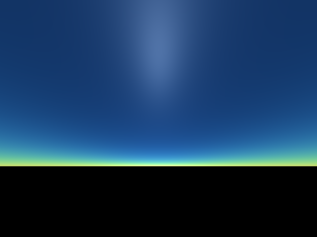
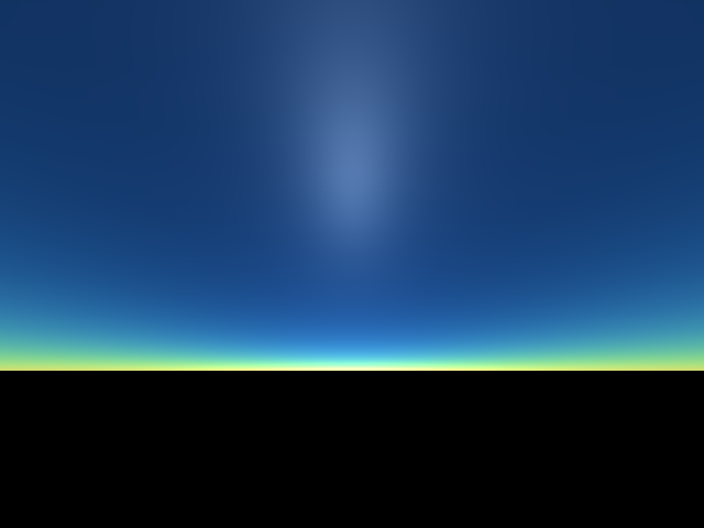
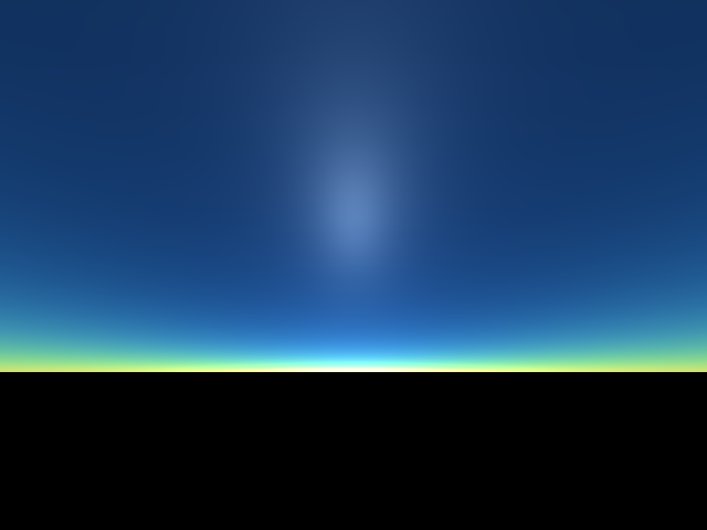
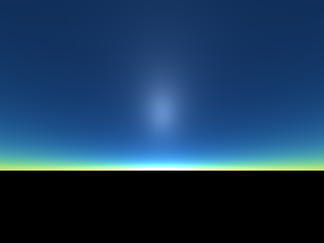
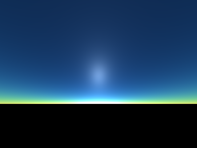
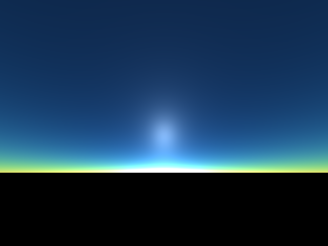
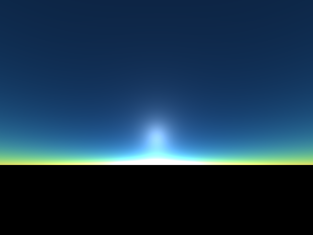
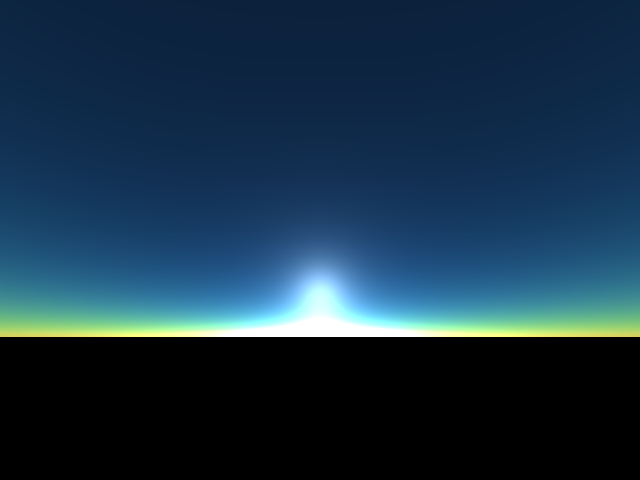
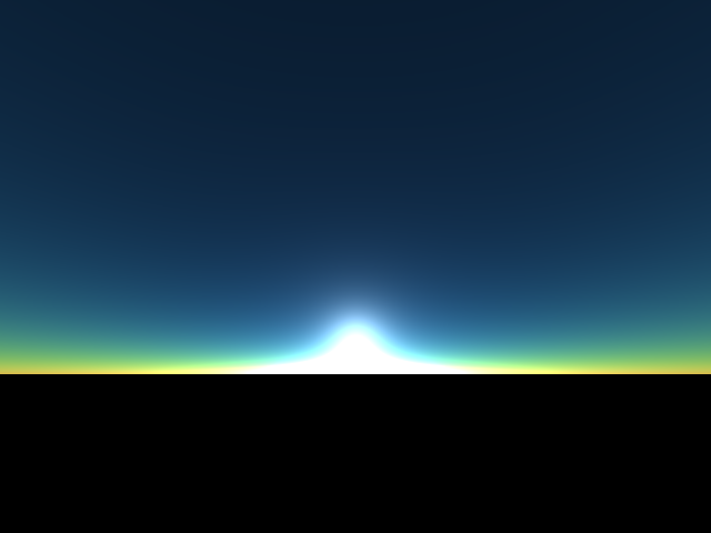
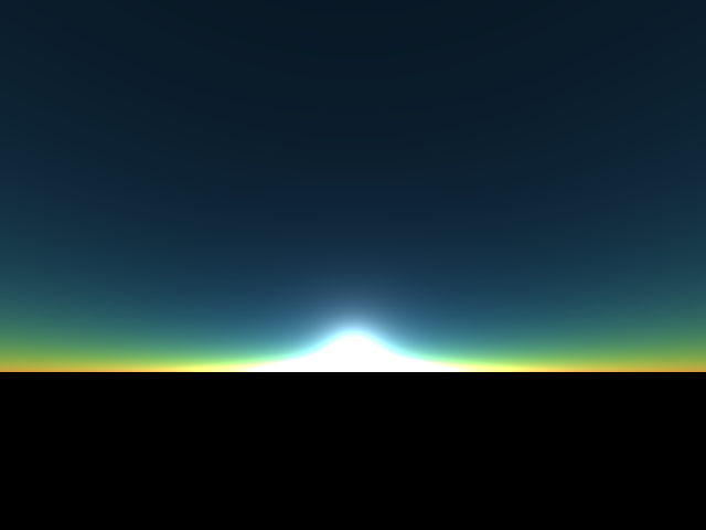
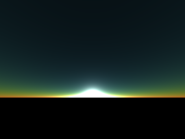
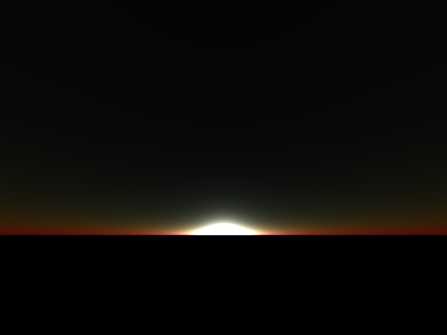
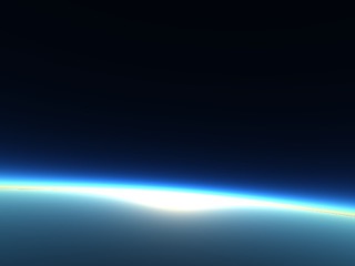
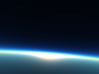
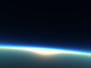
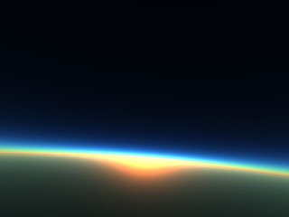
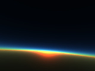
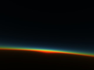
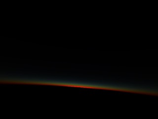
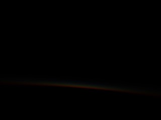
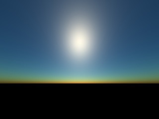
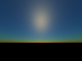
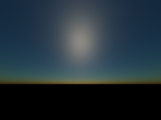
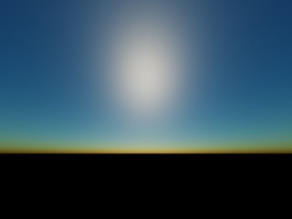
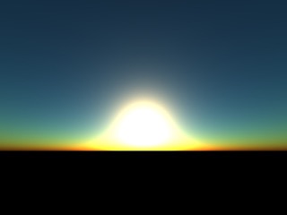
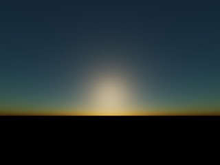
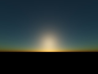
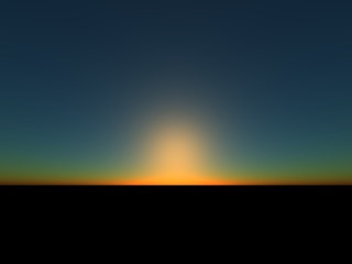
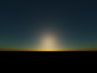
Volume Rendering: Results
Angle = 0.00
Angle = 6.07
Angle = 12.13
Angle = 18.20
Angle = 24.27
Angle = 30.34
Angle = 36.40
Angle = 42.47
Angle = 48.54
Angle = 54.61
Angle = 60.67
Angle = 66.74
Angle = 72.81
Angle = 78.88
Angle = 84.94
Angle = 91.01
Angle = 97.08
Angle = 103.15
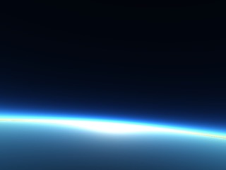
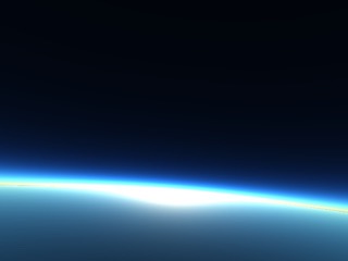
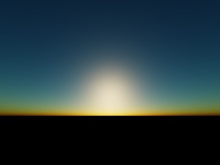
Since we've built a physical model, we can render images from different perspective by a simple change of camera position.
Below are rendered with camera located at x = 500000, above atmosphere.
Angle = 72.81
Angle = 75.24
Angle = 77.66
Angle = 80.09
Angle = 82.52
Angle = 84.94
Angle = 87.37
Angle = 89.80
Angle = 92.22
Angle = 94.65
Angle = 97.08
Angle = 99.51
Tone Mapping: Technical Approach
In reality, the luminance of the sky can be arbitrarily high, with values in the range of $[0, \infty)$ at each
point.
However, computer screens have limited display capabilities and can only show RGB colors within the range of
$[0, 255]$.
As a result, any values above 255 will be clipped during rendering, resulting in a loss of detail.
To address this problem, we use tone mapping, a mathematical technique that maps values from the high dynamic
range (HDR) of $[0, \infty)$ to the low dynamic range (LDR) of $[0, 255]$.
In our project, we have experimented with several tone mapping techniques.
Reinhard
This is one of the simplest tone mapping operator. It is calculated as: $$L_{out} = \frac{L_{in}}{L_{in} + 1}$$
Extended Reinhard
Standard Reinhard tone mapping does not utilize the full range of our Low Dynamic Range. Extended Reinhard takes
into account of the brightest radiance in our image and maps that value to $(1.0, 1.0, 1.0)$.
We define the brightest luminance as $L_{white}$. Extended Reinhard tone mapping equation is as follows:
$$L_{out} = \frac{L_{in}}{1 + \frac{L_{in}}{L_{white}^2}}$$
Extended Reinhard (Luminance Tone Mapping)
The above TMO operates on individual color channel instead of total luminance, but luminance is also an
important part of how an image appears.
A color value might be the same, but they will appear brighter. For example, (0.0, 1.0, 0.0), green, appears
brigher than (0.0, 0.0, 1.0), blue.
Luminance tone mapping a technique that takes luminance into account.
The equation is given by: $$L_{out} = L_{in} \frac{Lum_{in}}{Lum_{out}},$$ where Lum is calculated as: $$ Lum =
0.2126R + 0.7152G + 0.0722B$$
Uncharted Filmic Tone Mapping
The filmic tone mapping curve is another technique commonly used. It differs from reinhard TMO as it is based on
a more complex model of human vision,
which takes into account phenomena such as color adaptation and contrast sensitivity.
It is calculated as follows:
$$L_{out} = \frac{L_{in} * (A * L_{in} + C * B) + D * E}{L_{in} * (A * L_{in} + B) + D * F} - \frac{E}{F}$$
for uncharted2, the basic parameters are defined as:
A
B
C
D
E
F
0.15f
0.50f
0.10f
0.20f
0.02f
0.30f
Approximate ACES (Academic Color Encoding System)
This is another commonly used filmic tone mapping. We use the simplified, approximate version by Krzysztof
Narkowicz.
It is calculated as:
$$L_{in} *= 0.6$$
$$L_{out} = \frac{L_{in} * (A * L_{in} + B)}{L_{in} * (C * L_{in} + D) + E}$$
the parameters are defined as:
A
B
C
D
E
2.51f
0.03f
2.43f
0.59f
0.14f
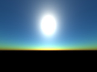
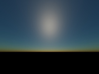
Tone Mapping: Results
Here are our results, we included the image rendered with no mapping tone for reference.
Sequence 40, sun angle = 48.54.
No Tone
Reinhard
Extended Reinhard
Reinhard with Lum
uncharted2
ACES approx
Sequence 60, sun angle = 72.81.
No Tone
Reinhard
Extended Reinhard
Reinhard with Lum
uncharted2
ACES approx
ChatGPT has also given us their own tone mapping.
From this cartoon like gif, we are able to see the power of tone mapping.
Through a simple function, the appearance of an image can be dramastically changed.
A Peak into Real-Time Rendering
The rendering time of our scene significantly increases as we increase the number of samples on camera ray (V)
and/or light source ray (L),
as well as the image size.
Below is a comparison table highlighting the substantial increase in render time.
Width
Height
Num of Samples on V
Num of Samples on L
Average Render Time
640
480
16
8
3.5593s
1900
1000
100
50
323.926s
Sky rendering is a crucial aspect of game engines,
but as seen above, it is highly computationally expensive.
To address this challenge, we explored various techniques to improve rendering speed.
One common approach used in the industry is precomputing a lookup table,
where L values are calculated in advance for each camera location and viewing direction.
Due to time constraints, we simplified the problem by fixing the camera location and only computing a lookup table
for varying viewing directions.
We create three seperate maps representing the three color channels,
and the first three values within each map are keys to specify a viewing direction.
Our maps for width = 1900, height = 1000, num of samples on V = 100, num of samples on L = 50, sun angle = 0
can be found here:
Lookup Table
Normal Render
Render with lookup table
We observed a significant improvement in rendering runtime,
but it still falls short of real-time requirements.
Achieving real-time rendering would require GPU parallelism or other advanced tools,
which we were unable to implement within our project timeline.
Width
Height
Num of Samples on V
Num of Samples on L
Average Render Time
1900
1000
100
50
6.2582s
Rainbow, or Halo?: Technical Approach
We found a
guide provided by
Nvidia on rendering rainbows and other natual effects caused by waterdrops in the air. Rainbows (and Halo) is caused
by refractions of light with different wavelength
inside the water droplet. The color of the rainbow is determined by the angle of deviation (angle between the eye and
the sunlight) and radius of the waterdrop. A Lee diagram
provides a precomputed texture. With a precomputed lookup table for rainbow color, we were able to sample the lookup
table as a texture, and blend the sampled color with the computed
sky color. The X-axis of the lookup table is the radius of the water droplet, which we could determine based on the
different visual effects we want, and the Y-axis
of the lookup table is the angle between the sun direction and the view direction (our camera ray direction).
While the conceptual ideas were simple, this tutorial provided by Nvidia was intended for shaders, and the terminology
it used were all for vertex shaders. We adapted the methods
described in the article for a brute force calculation within our rendering function. After calculating the color of
the pixel, we then use the camera ray projected by this pixel
and viewing direction, and proceed to the texture map to query the color at this pixel location.
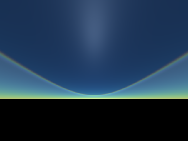
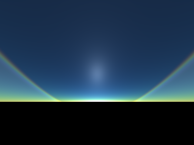
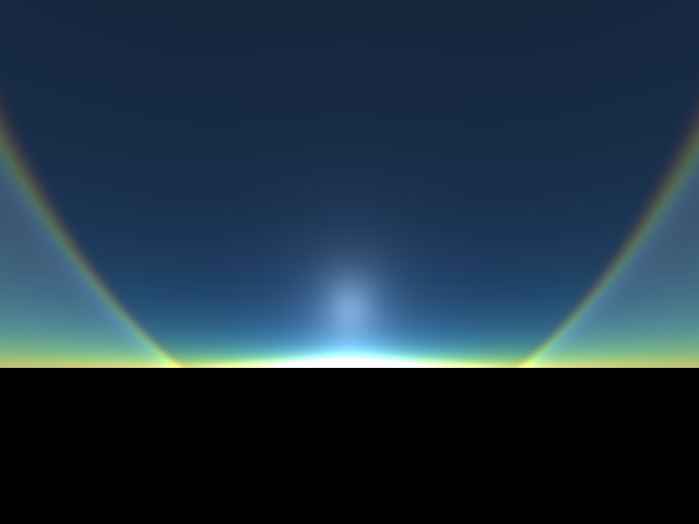
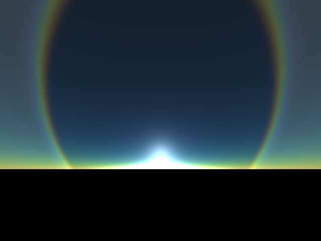
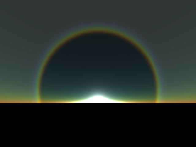
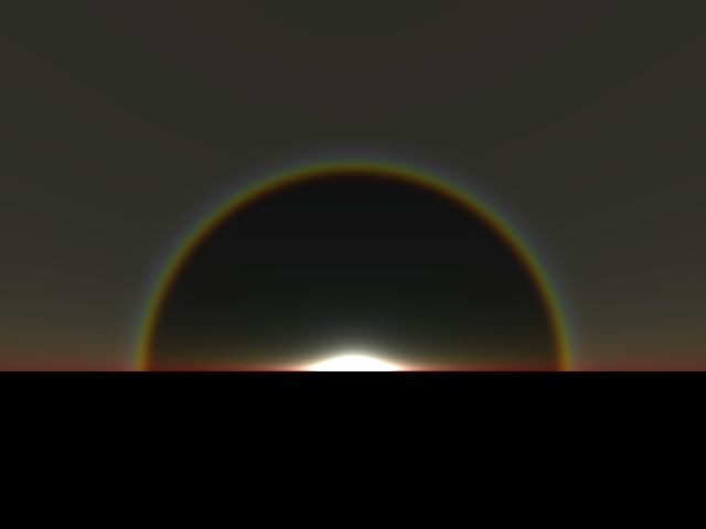
After rendering the results, we are actually a bit confused if we are rendering halo or rainbow, because halo is
circular around
the sun, and rainbow is more like an arch. (but it looks good either way)
Rainbow, or Halo?: Results
hmm, so is this halo or rainbow?
Angle = 24.27
Angle = 48.54
Angle = 60.67
Angle = 72.81
Angle = 84.94
Angle = 91.01
Problems Encountered in Implementation
We had a LOT of troubles understanding the physics and math behind the scene, especially the integration. While it
took a while to understanding the conceptual integration,
it took us even longer to understand the Ray-marching algorithm described by Scratchapixel.
We even had a shared page
where we write down our understanding of the tutorials and the paper.
We were also having troubles with implementing our ideas using C++. For the rainbow section, the conceptual idea
of sampling a texture was very simple, but it took us a long time to finally load
the texture using C++. We spent hours reading OpenCV documentation for C++ and also tried the library used by
staff for Project 4, the stb_image library.
Lessons Learned
Learning about the physics behind the sky was very interesting, and when we finally understood it, it was very
fulfilling.
We also regret not using Python for the project. We used C++ because we've been using C++ throughout the semester,
but C++ was so painful, and for the purpose of our project (simulating rays to calculate pixel color), we could
have used Python. In addition, since
our project was not built on top of existing class projects, we were able to directly borrow the staff code. So
when I tried to borrow code from class projects, it took me an hour to realize that CGL was a custom
library written by the staff, and we were NOT using OpenGL directly!
Resources
For simulating the sky:
Scratchapixel. (n.d.). Simulating colors of the sky. https://www.scratchapixel.com/lessons/procedural-generation-virtual-worlds/simulating-sky/simulating-colors-of-the-sky.html
Nishita, T., Nakamae, E., Miyawaki, Y., & Shinya, M. (1993). A display method of the earth taking into account atmospheric scattering. SIGGRAPH '93 Proceedings of the 20th annual conference on Computer graphics and interactive techniques, 175-182. http://nishitalab.org/user/nis/cdrom/sig93_nis.pdf
Bruneton, E., & Neyret, F. (2008). Accurate atmospheric scattering. GPU Gems 2, 175-198. https://developer.nvidia.com/gpugems/gpugems2/part-ii-shading-lighting-and-shadows/chapter-16-accurate-atmospheric-scattering
Habel, R., Kuhlen, T., & Dachsbacher, C. (2020). Real-time rendering of atmospheric phenomena using voxel cone tracing. Computer Graphics Forum, 39(4), 107-119. https://sebh.github.io/publications/egsr2020.pdf
For the rainbow:
Bruneton, E., & Neyret, F. (2008). Accurate atmospheric scattering. GPU Gems 2, 175-198. https://developer.nvidia.com/gpugems/gpugems2/part-ii-shading-lighting-and-shadows/chapter-16-accurate-atmospheric-scattering
For tone mapping:
Tayler,M. Tone Mapping. https://64.github.io/tonemapping/
For real time rendering:
Boubekeur, T., & Schlick, C. (2008). Efficient evaluation of functions defined by distance fields. In Proceedings of the 2008 ACM symposium on Solid and physical modeling (pp. 87-98). https://hal.inria.fr/inria-00288758/document
Code are in C++.
Contributions
Zhihan Cheng: Implemented sky rendering, tone mapping, real-time rendering, wrote final Report, recorded video
Yuerou Tang: Implemented sky rendering, rainbow, wrote final report, recorded video
Long He: Implemented sky rendering, rainbow, wrote final report, recorded video
Debby Lin: Wrote proposal
Gallery
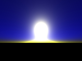
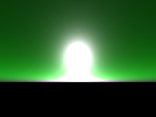
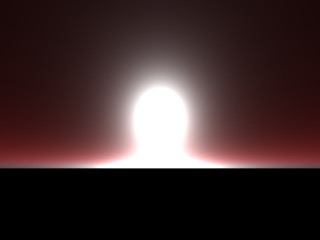
This is what the sky could look like is only certain wavelength can be reflected.
Only 440nm Scattering
Only 550nm Scattering
Only 680nm Scattering
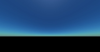
Rayleigh scattering occurs when light interacts with small particles in the atmosphere,
such as nitrogen and oxygen molecules.
This type of scattering is responsible for the blue color of the sky during the day,
and the red and orange colors seen during sunrise and sunset.
This is because shorter-wavelength blue light is scattered more than longer-wavelength red and orange light.
On the other hand, Mie scattering occurs when light interacts with larger particles in the atmosphere,
such as dust, smoke, and water droplets.
This type of scattering is responsible for phenomena such as haze and fog.
Only Rayleigh Scattering
Only Mie Scattering
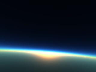
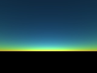
This image of a sunset was created by stitching together 90 individual images,
each taken with a different sun angle.
The result is the view of the sun setting over the horizon. The image was not tone mapped.