|
|
|
For this project, we implemented a real-time cloth simulation system. We used point masses and springs to represent the cloth and applied physics of motion (forces) to the different point masses in the cloth to represent movement. We then implemented support for simulation by using Verlet integration to calculate new time steps and to compute new point mass positions. To avoid deformation in our cloth, we also implemented constraints for position updates for each time step. Next, we add support for handling the cloth’s collision with other objects such as spheres and planes, and also support for self-collision to avoid clipping. We implement self-collision support by using a hash table for efficient lookup of whether certain point masses collide with each other. Finally, we write shaders to accelerate rendering of our cloth with different materials. At the end, we now have a working real-time cloth simulator that realistically simulates cloth with physics and that also supports different cloth materials.
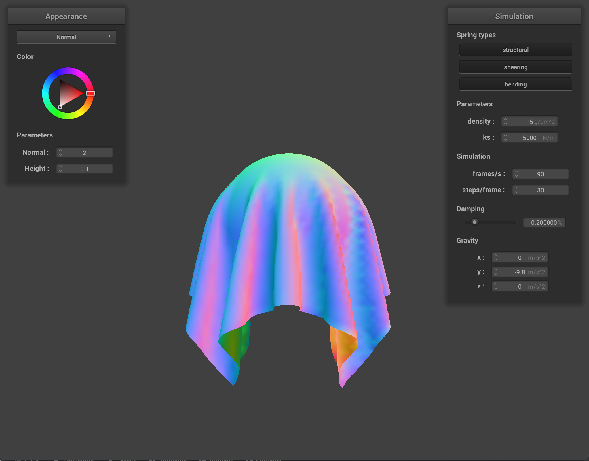
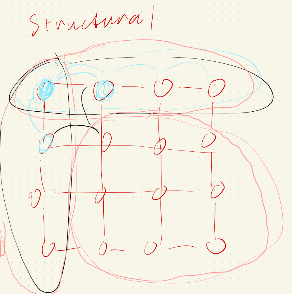
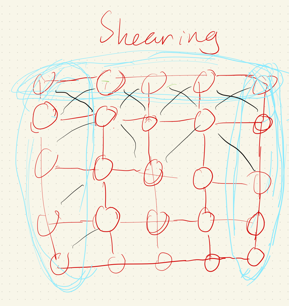
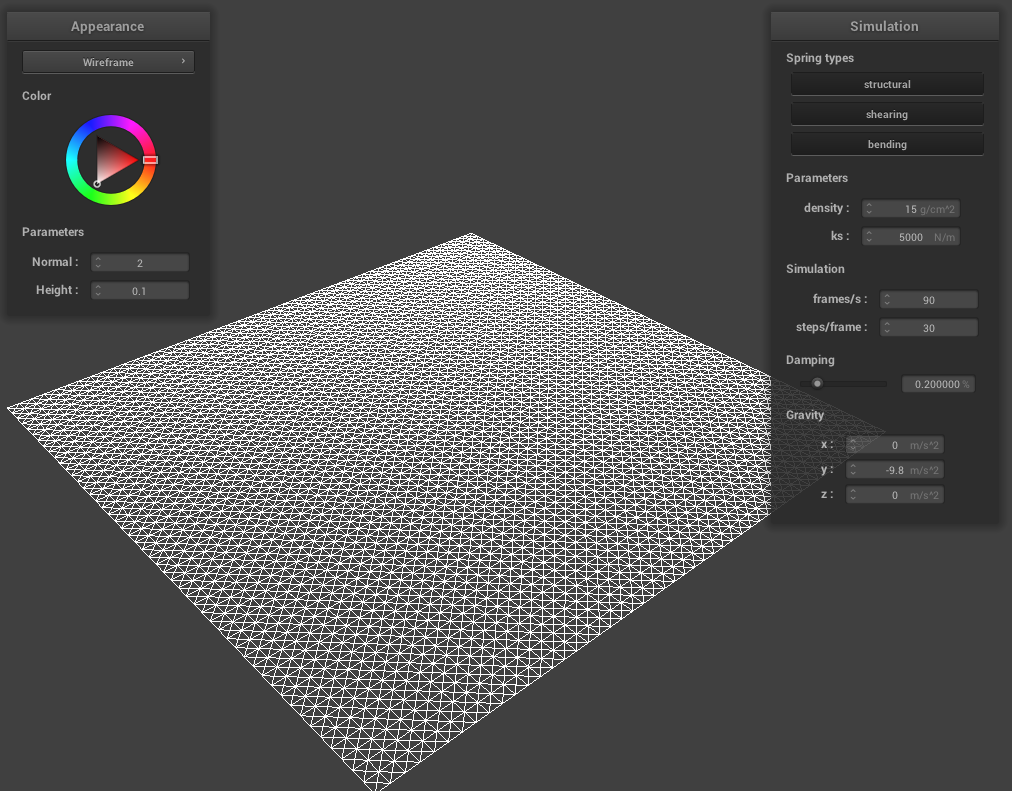
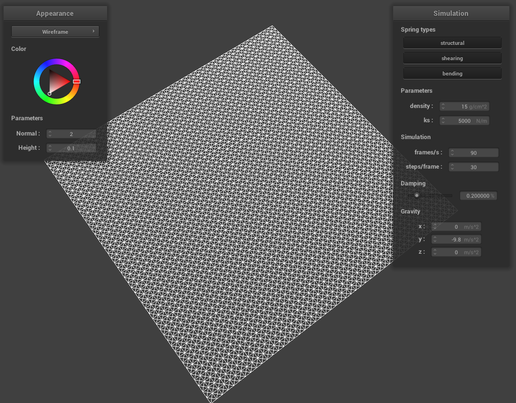
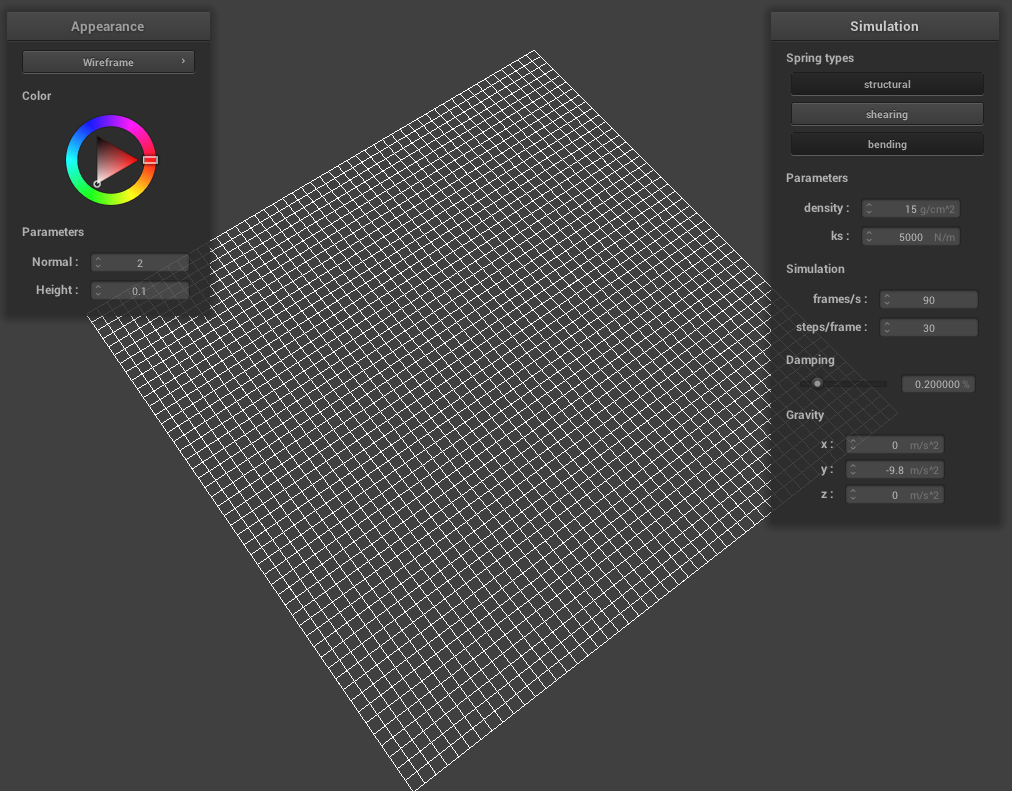
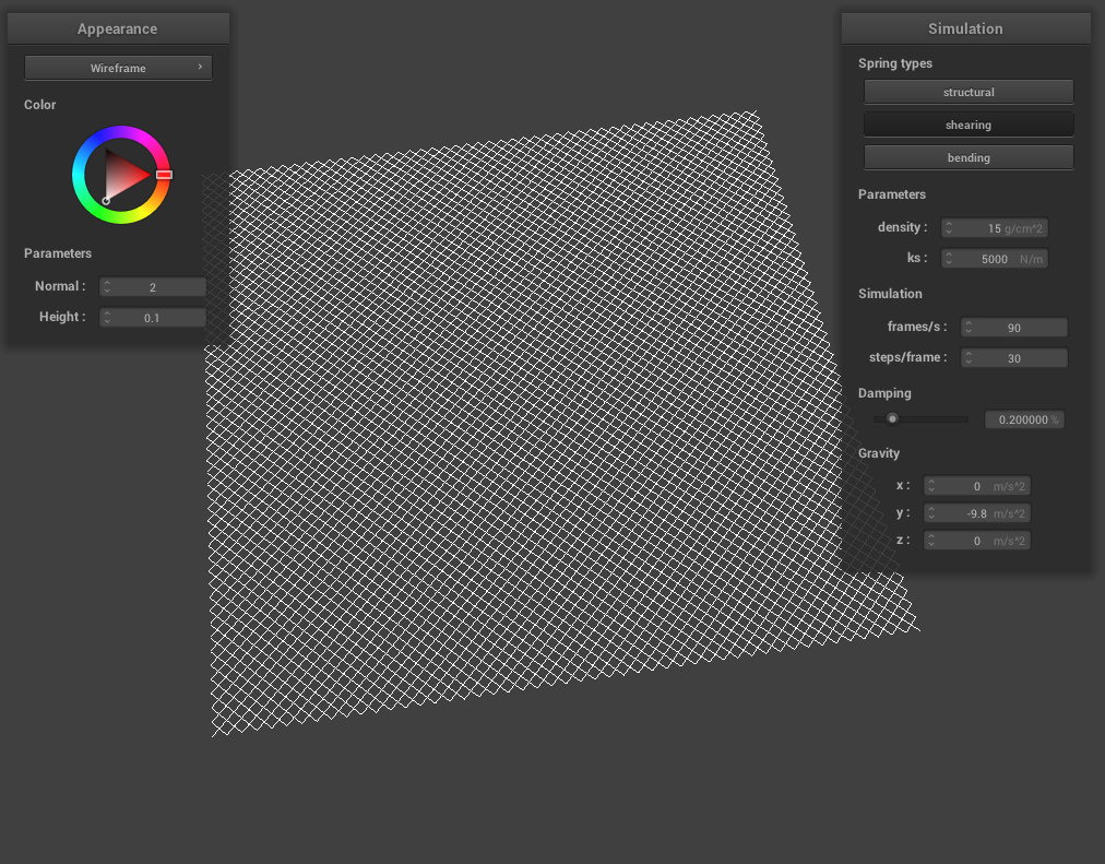
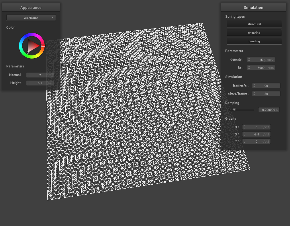
Throughout this project, we use a system of point masses and springs to represent our cloth model. We divide the cloth with evenly spaced point masses and connect each point mass with the proper spring type(s). To begin implementing this system, in Cloth::buildGrid(), we first start by creating the evenly space point masses grid. We take into account the cloth’s orientation (horizontal or vertical, in which case we vary positions over the xz plane or xy plane respectively) while iterating through num_height_points and num_width_points for the total number of masses, create a new PointMass that takes in the position we calculated and set our pinned boolean to false (we will go back later to adjust this), and store all the point masses in the point_masses vector using emplace_back() in row-major order. Once we have a grid of all our point masses, we iterate through our point_masses vector to set whether a point mass is pinned according to the indices contained in our pinned vector (if the index is found within the pinned vector, then that means our point mass for that specific index is pinned and we should change the pinned boolean to true). Then, we create our three spring types: structural, shearing, and bending. To figure out how to implement these springs, we drew diagrams to figure out edge cases for each spring type. For shearing springs, springs exist diagonally between point masses (diagonal upper left and diagonal upper right). Structural (exists between a point mass and the point mass to the left and directly above) and bending (exists between a point mass and the point mass two to the left and and two directly above) springs are a bit more similar in the sense that they exist horizontally and vertically between point masses. To create each of the springs once we have our edge cases figured out, we iterate through all the point masses and create a new spring with the corresponding point masses on either end of the spring, as well as the type of spring it is. Using emplace_back(), we then store our created springs into the springs vector.
|
|
|
|
|
|
|
|
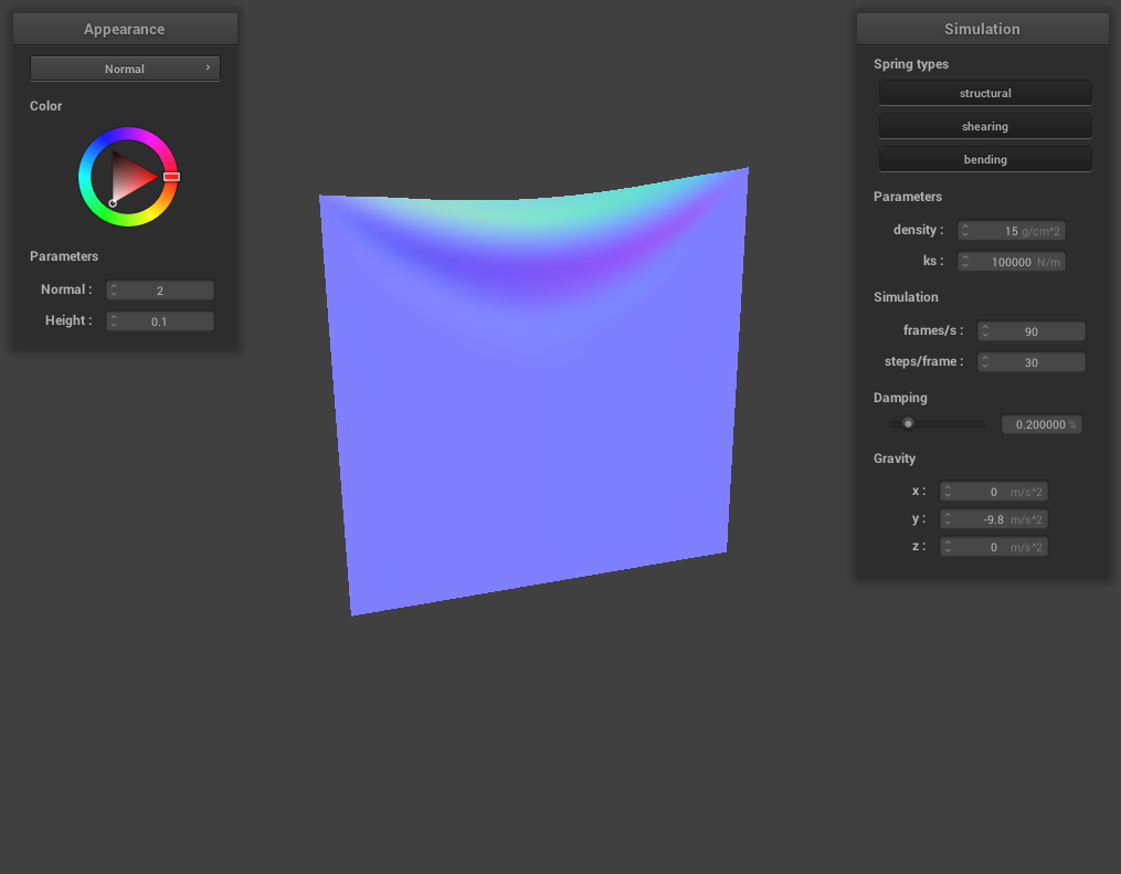
To simulate our cloth, we need to implement some physics to represent motion in our cloth model. In Cloth::simulate(), we apply two types of forces (external forces such as gravity and spring correction forces, which both make up our total forces) on our cloth point masses in order to represent movement from one time step to the next. We first start by computing the external forces on each point mass. We do this by iterating through external_accelerations, which contains all our external forces, and multiply each external force by a mass (F=ma), which we then store/accumulate in each respective point mass’s forces vector. Next, we calculate the spring correction forces by iterating through each spring in the springs vector, checking if the specific spring’s constraint type is enabled (using ClothParameters pointer) and if the spring type corresponds to the constraint type. If true, then we can calculate the spring correction forces. We first use Hooke’s law to compute the force F_s applied to the ends of two point masses. In Hooke’s law, k_s represents the spring constant, p_a and p_b are the positions of the point masses on either end of the spring, || means we’re taking the magnitude, and l is the spring’s rest length. Since the bending constraint is weaker than structural and shearing, we multiply the spring constant by 0.2. For accumulating the forces in each point mass, we multiply F_s by the unit vector of the two point masses’ position, making sure to acummulate an equal but opposite force to one point mass but not the other. We then use Verlet integration, one of the many methods of integrating equations, to go from one time step to the next and to compute the new point mass positions. In Verlet integration, x_t is the current position, v_t is the current velocity, a_t is the current total acceleration from all forces, d_t is a timestep, x_(t+dt) is the position in the next time step, x_(t-dt) is the position in the previous time step, and d is a damping term which helps to simulate loss of energy due to factors such as friction and heat loss. We iterate through each point mass and if a point mass isn’t pinned, then we update the point mass’s position and last position with the resulting values from Verlet integration. Finally, we apply a deformation constraint on our springs by adjusting/correcting the two point masses of a spring so the spring’s length isn’t greater than 10% of its rest length at the after any time step. We do this by first checking if the current length of the spring (which we obtain by subtracting one point mass’ position by the other and taking the norm) is greater than 1.1 times the spring’s rest length, which we then know we have some correction to do. There are a few conditions we consider here: if both point masses are pinned, then we don’t do anything, if one point mass is pinned, we apply a correction to the unpinned point mass’s position, and if both are unpinned, we apply half the correction to each point mass.
|

|
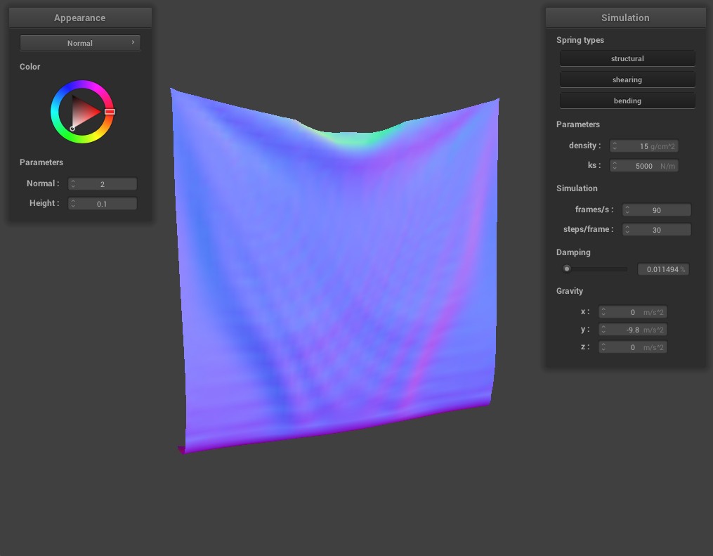
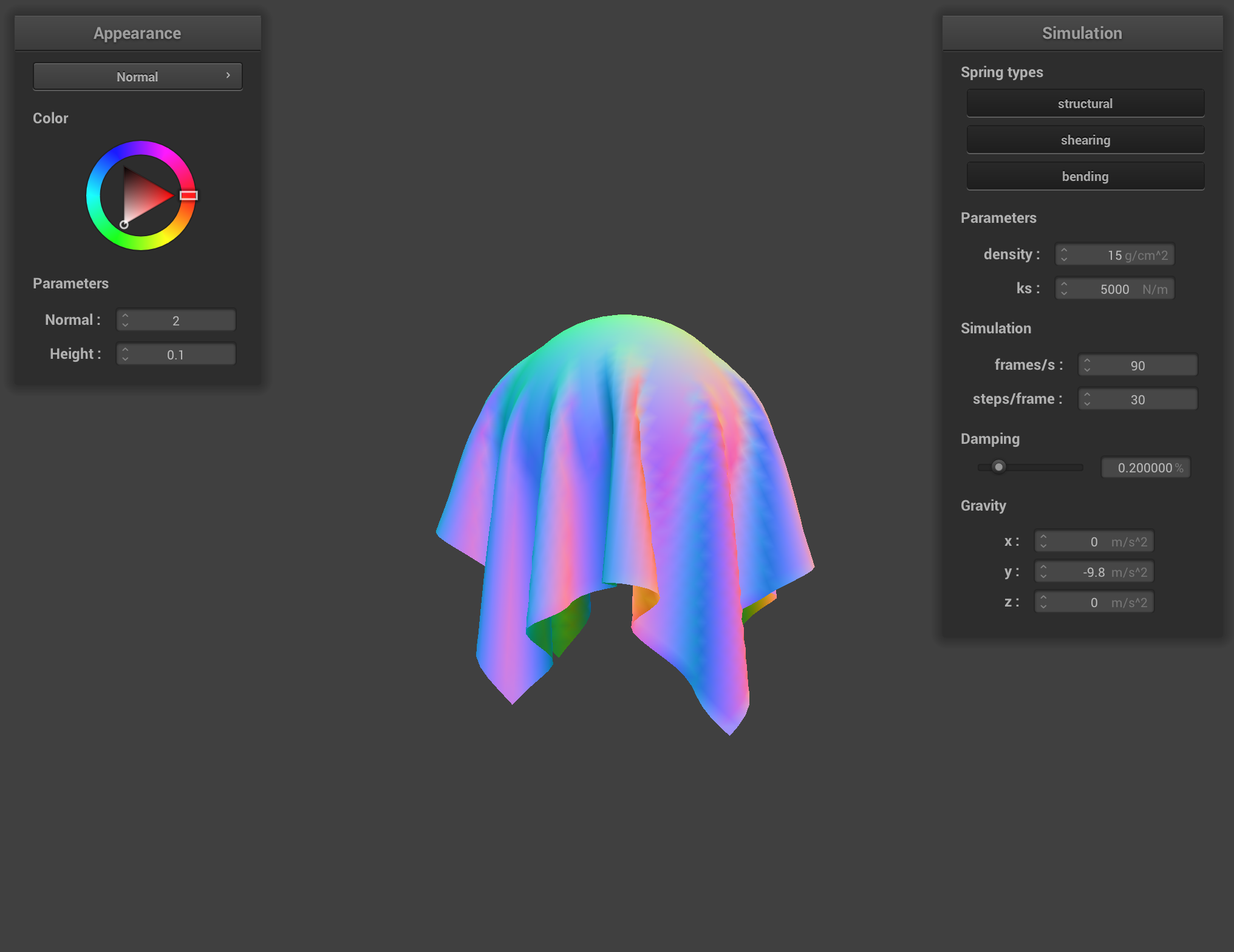
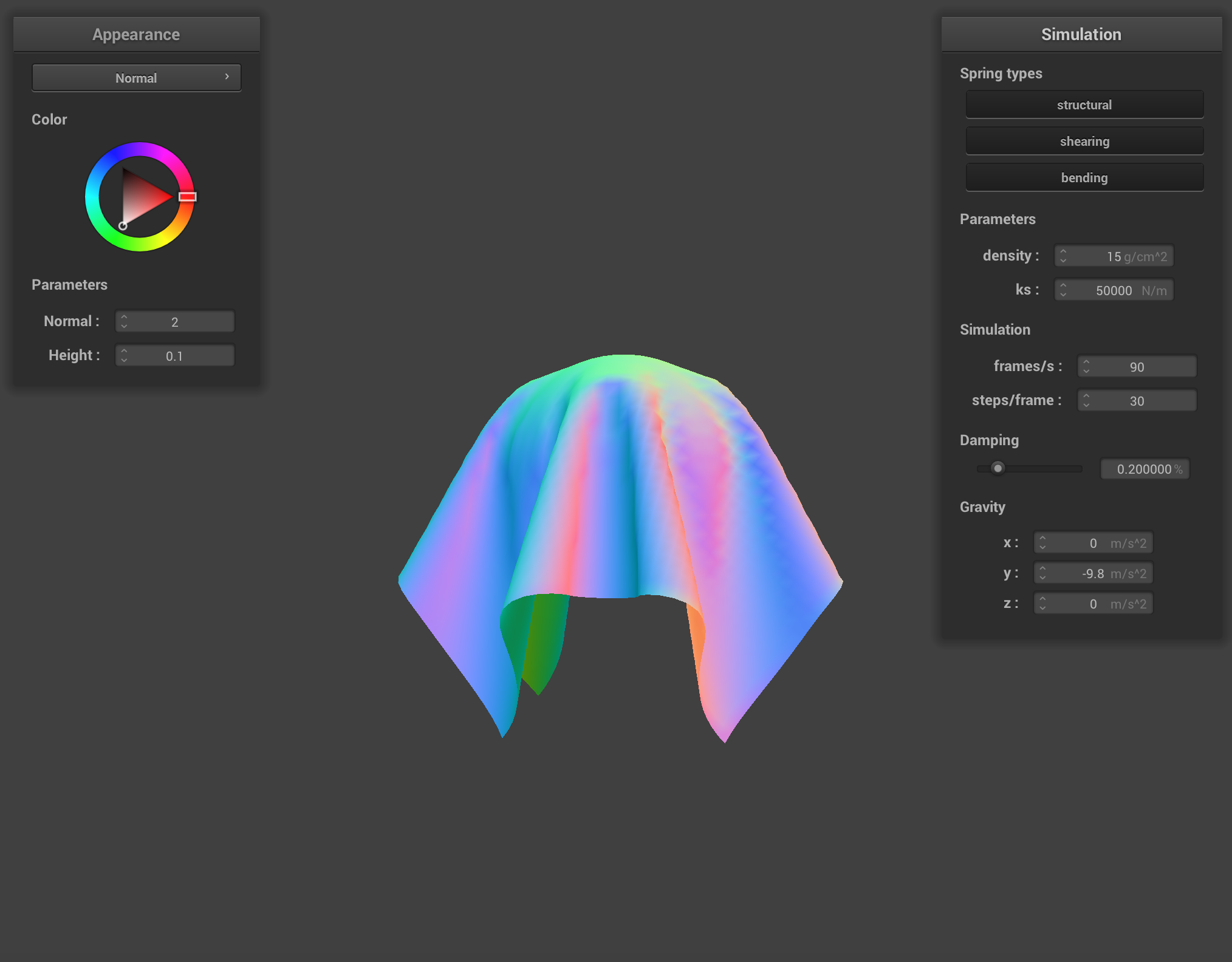
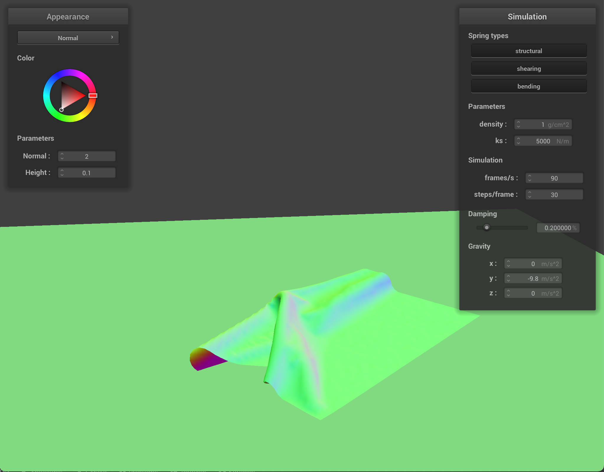
At a very low ks, the cloth appears to behave like a piece of thin, very stretchy fabric (for example, silk). It comes to a final resting state rather slowly and with many ripples throughout the cloth. At a high ks, the cloth appears stiffer with few ripples throughout the cloth as it reaches a final resting state. This makes sense because ks represents the spring constant and ks is directly proportional to the stiffness of a spring/object. This means a higher ks means the cloth is stiffer, while a lower ks means the cloth is more elastic/stretchy.
At a very low density, the cloth appears light or thin with little bounces (ripples present throughout though). At a high density, the cloth appears heavier and more weighed down (especially at the top of the cloth between the two pinned corners). This happens because density is the grams per square centimeter, which refers to the thickness of the cloth. When cloth is more dense, that means there is more cloth material in one square meter, compared to less dense cloth, giving the appearance of lighter and heavier cloth.
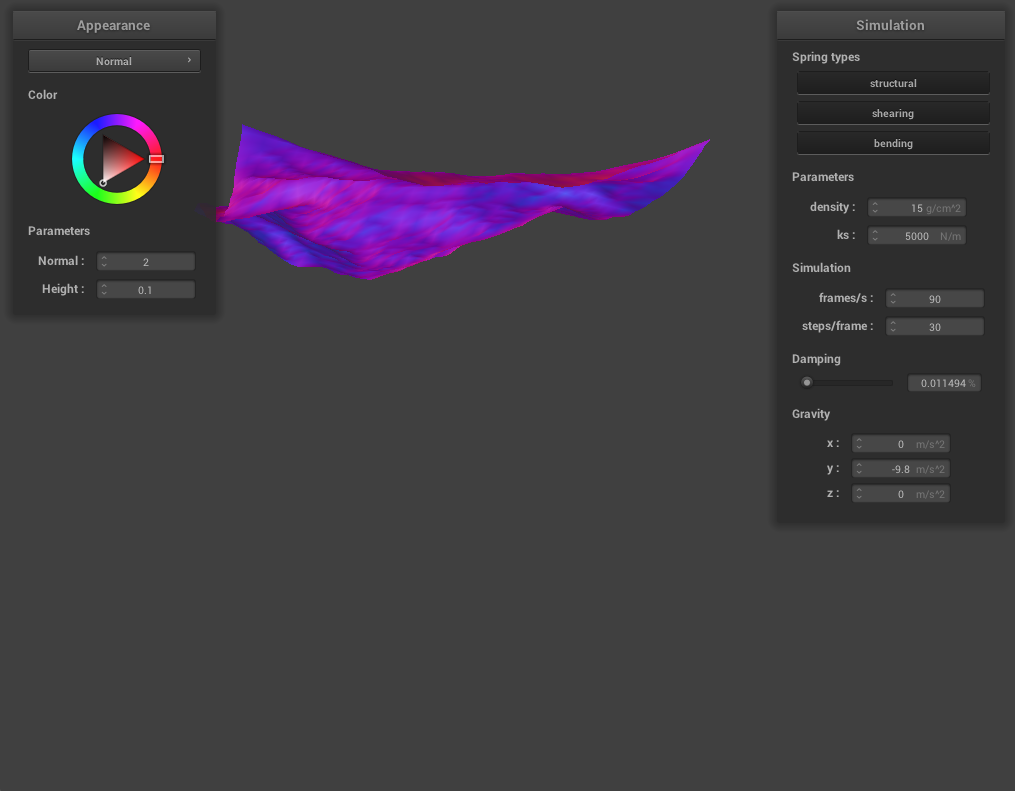
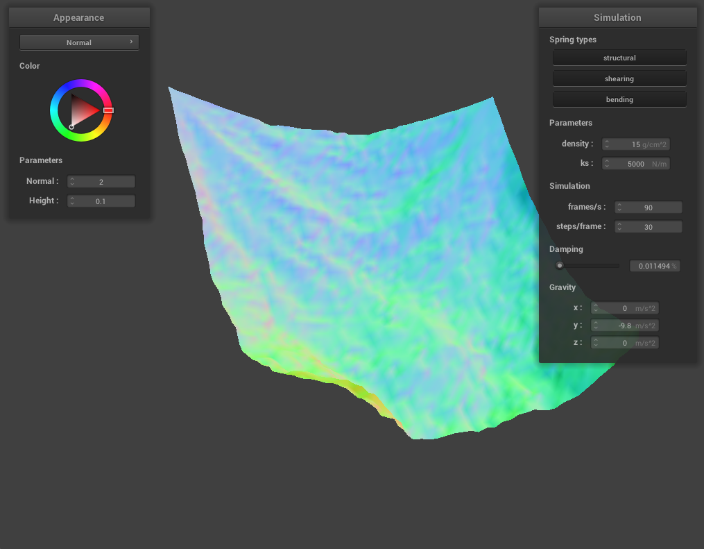
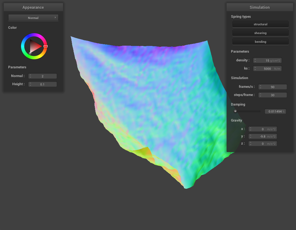
At a very low damping percentage, the cloth takes an extremely long time to converge to a final resting state, with many ripples, bounces, and even folding in on itself happening. At high damping, the cloth converges to a final resting state very quickly with little bouncing and rippling. This is because damping helps our cloth simulation represent loss of energy due to factors such as friction, heat loss, and other factors. At low damping, there is very little energy being lost at each time step which is why it takes a very long time for the cloth to reach a final resting state. At high damping, the energy loss is almost immediate and this can be seen with the cloth almost immediately coming to a final resting state.
|
|
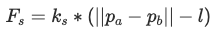
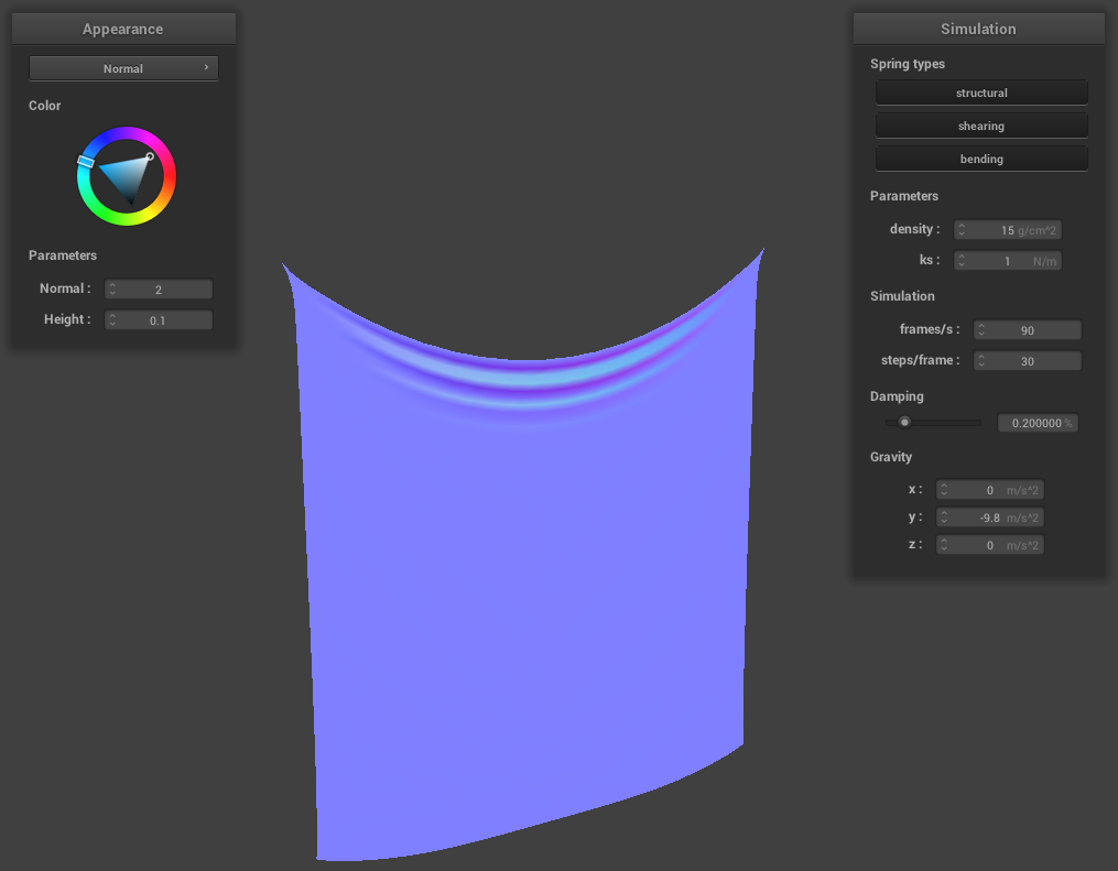
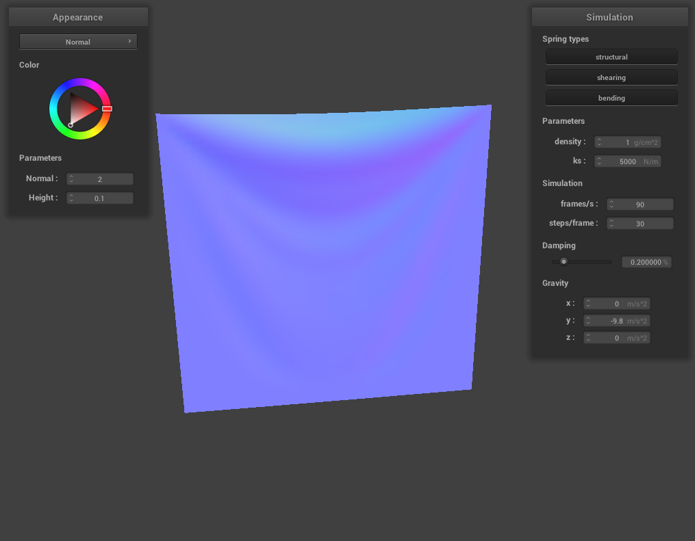
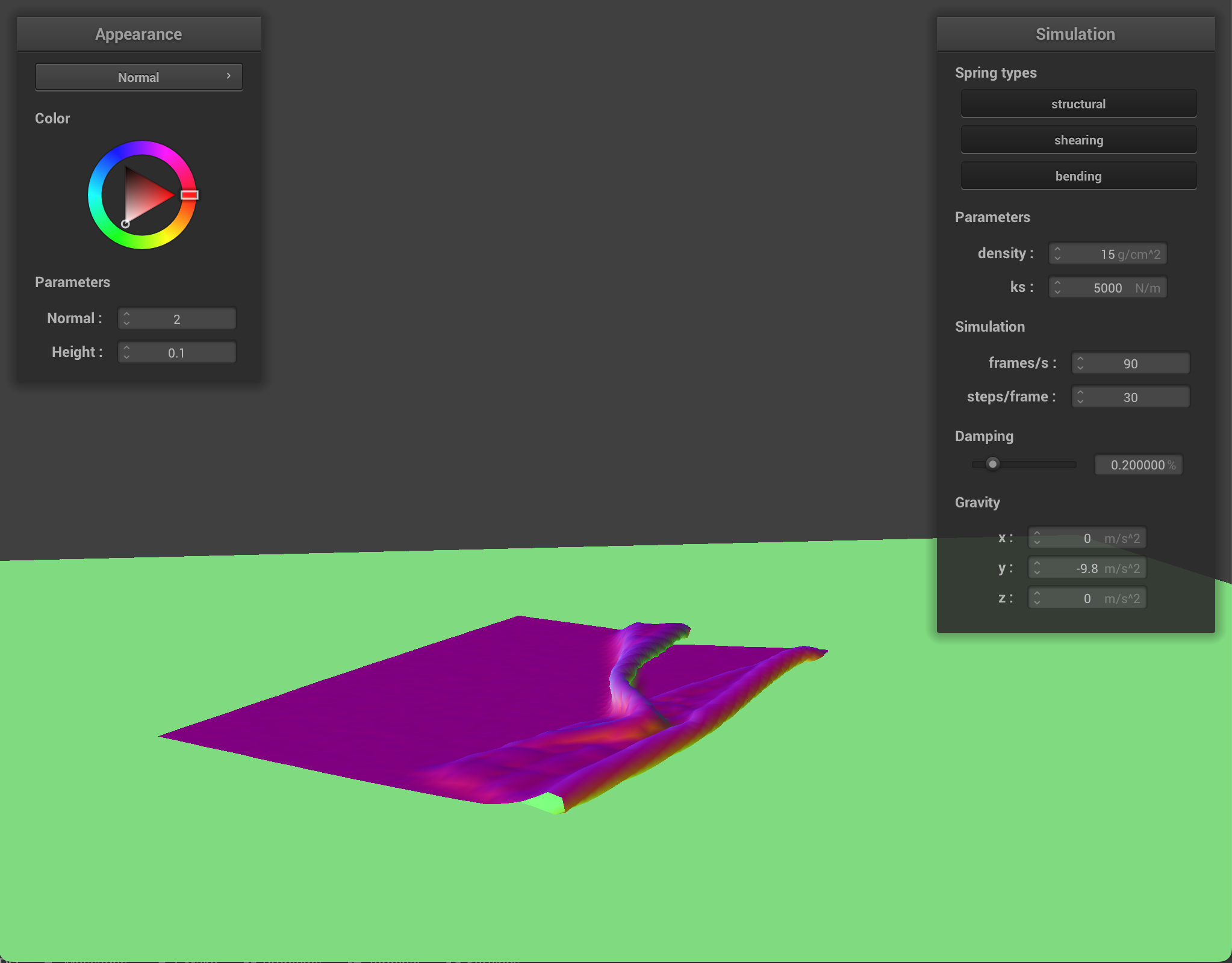
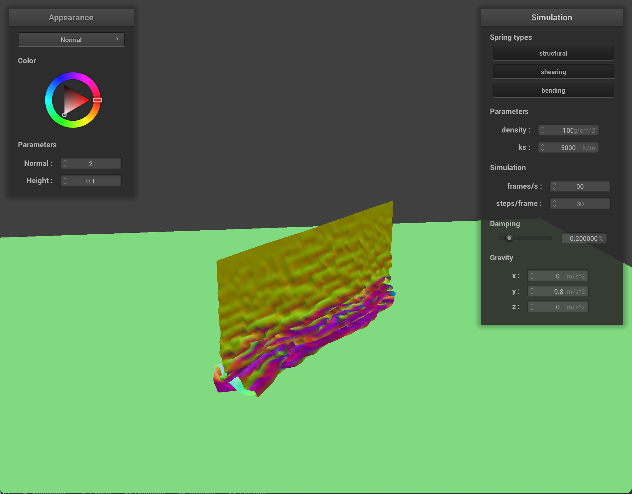
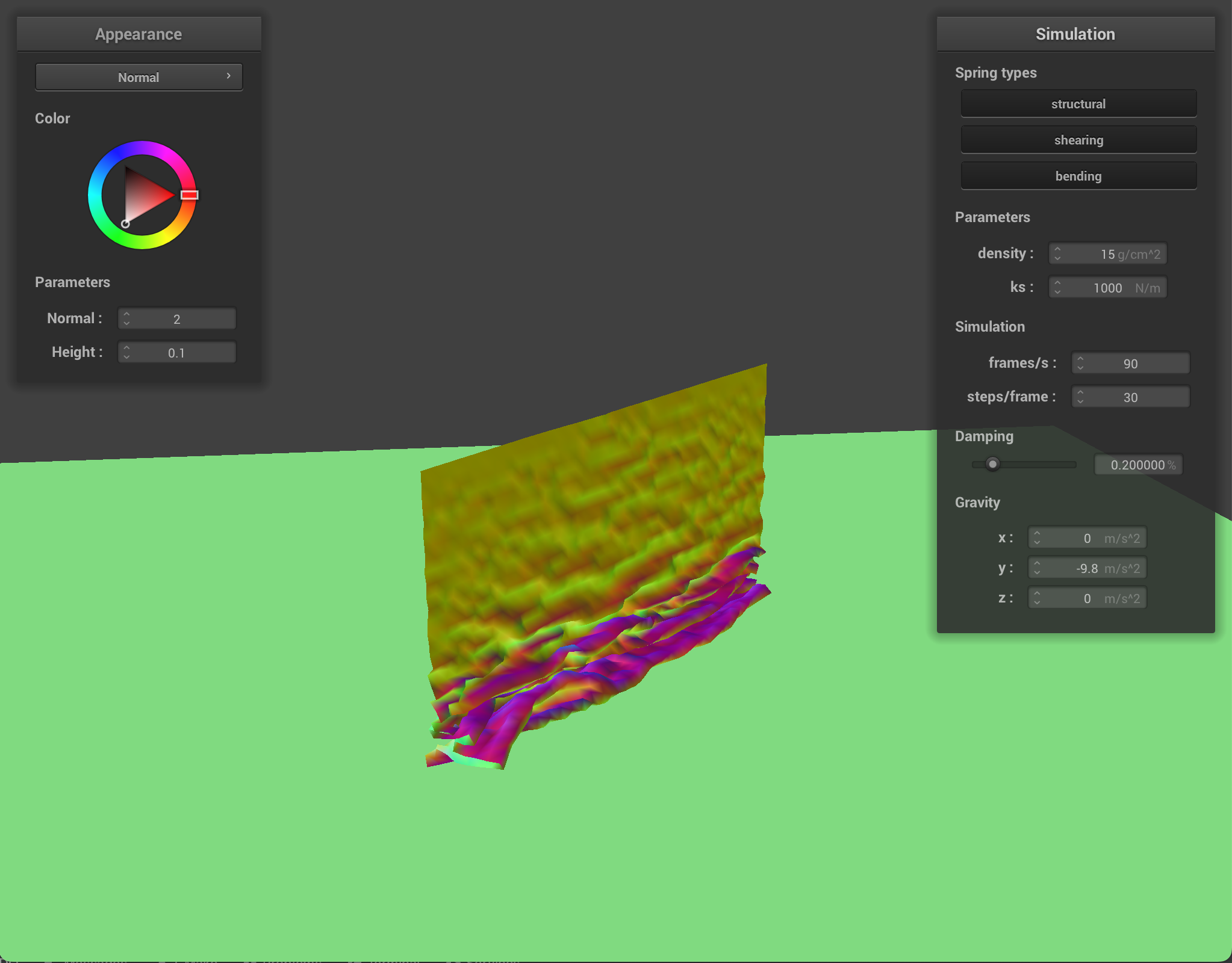
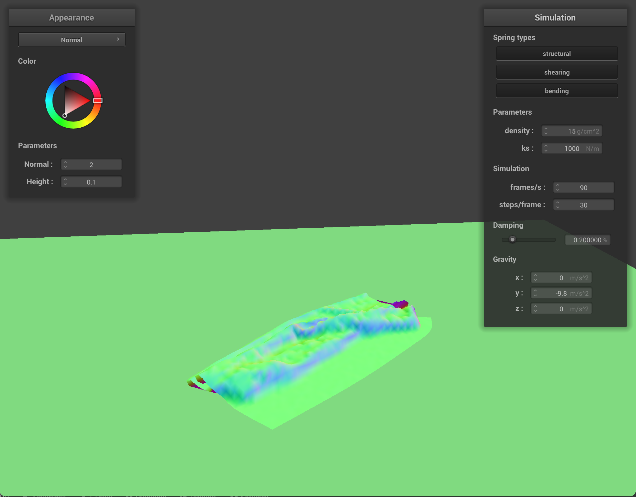
For ks, we experimented with ks = 1 N/m. There was a very noticeable difference compared to the default parameter of ks = 5000 N/m in that the fold at the top was very pronounced and there were no wrinkles throughout the cloth when the ks = 1 N/m. At ks = 5000 N/m however, the fold at the top wasn’t as pronounced and there were wrinkles throughout the cloth at its resting state. At a high ks = 100000 N/m, the cloth appeared much stiffer and there was very little folding at the top and with no wrinkles throughout. This makes sense because ks determines how stretchy/elastic cloth is and a low density of 1 N/m would mean the cloth is very elastic while a density of 100000 N/m would mean the cloth is very stiff.
|
|
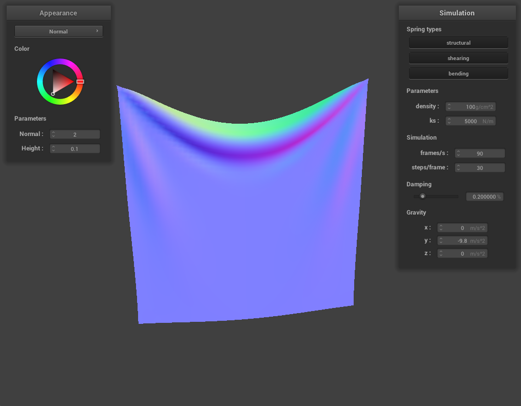
For density, we experimented with density = 1 g/cm^2 and density = 100 g/cm^2. There was a noticeable difference with density = 1 g/cm^2 in that the fold at the top was almost nonexistent, while the fold at the top for 100 g/cm^2 was even more pronounced than the default density parameter (15 g/cm^2). This happens because a low density of 1 g/cm^2 means the cloth is very light (hence little weight to make the fold at the top dip) and 100 g/cm^2 means the cloth is rather heavy.
|
|
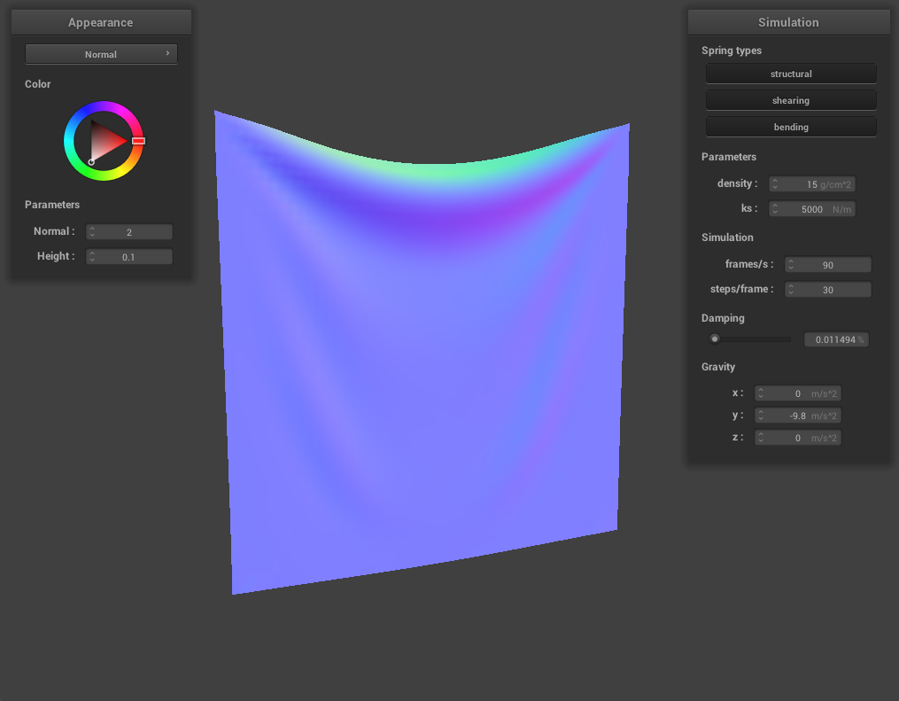
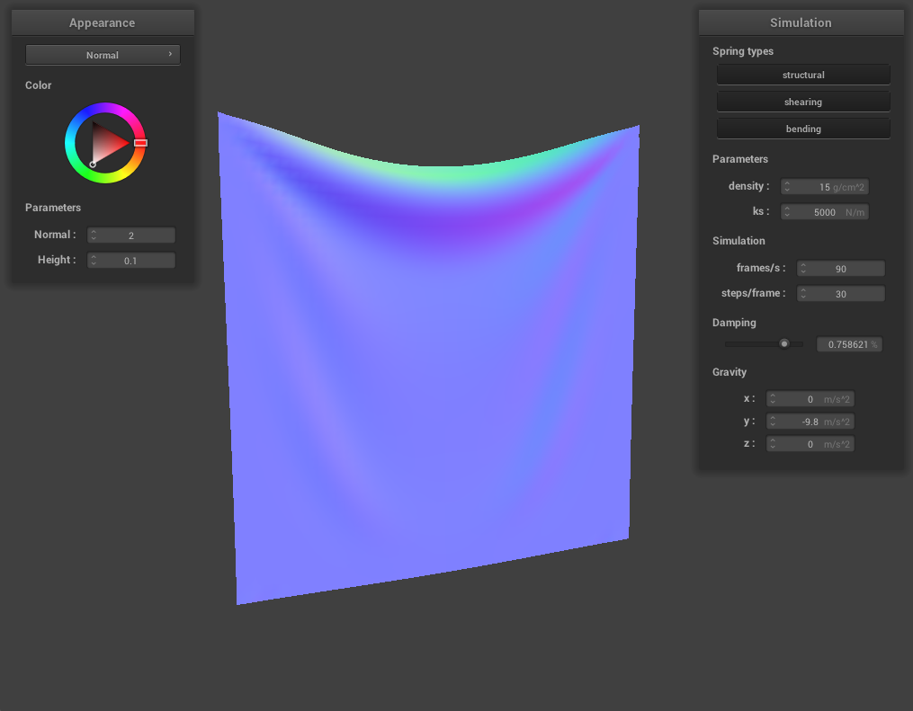
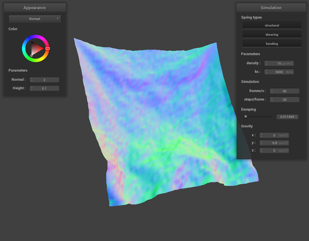
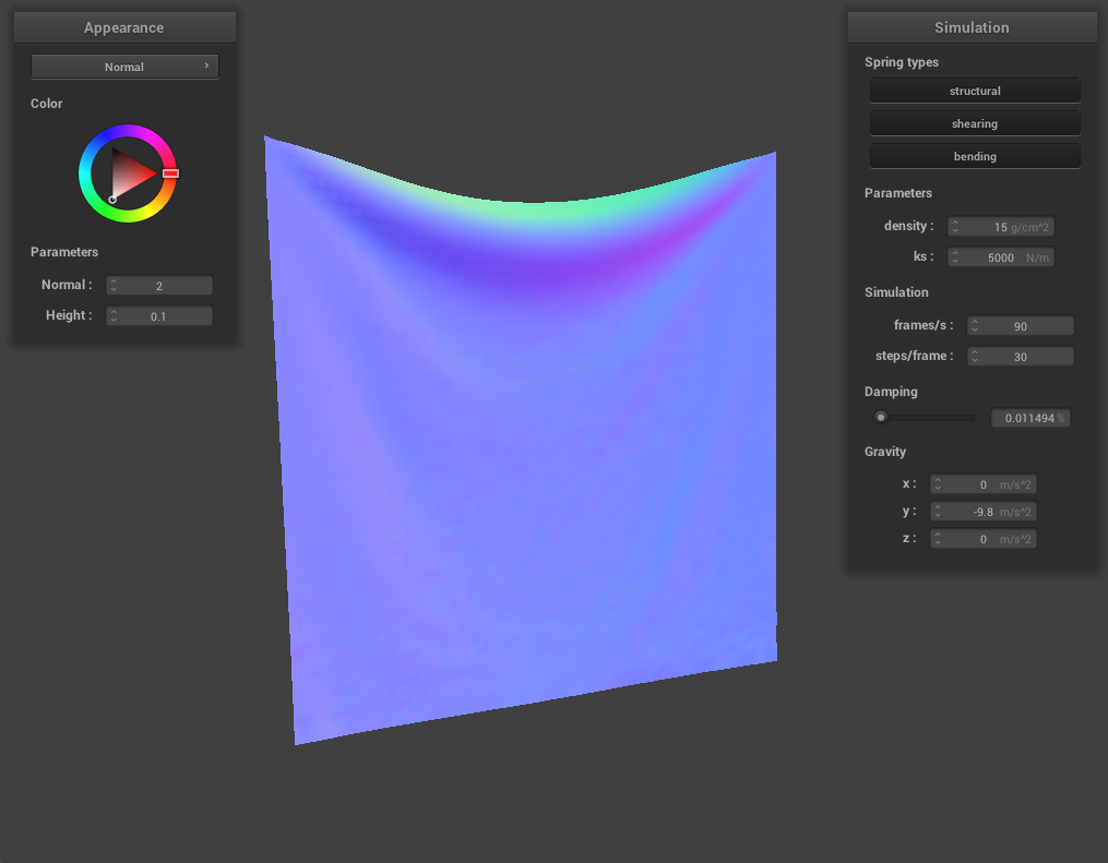
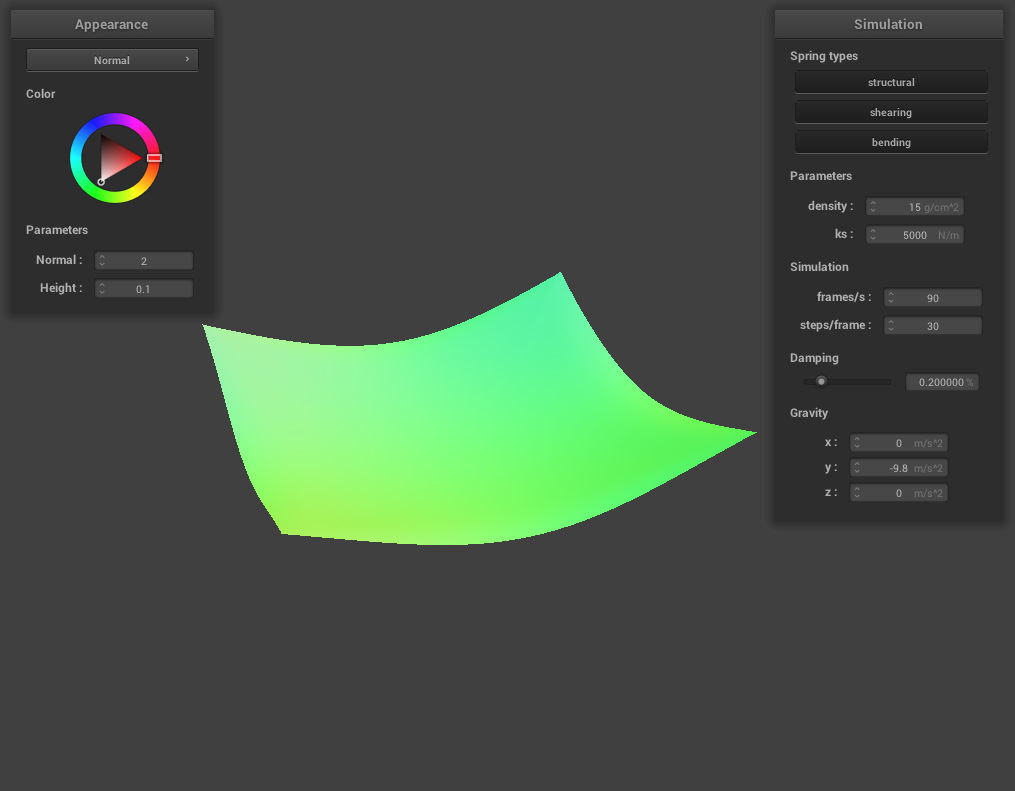
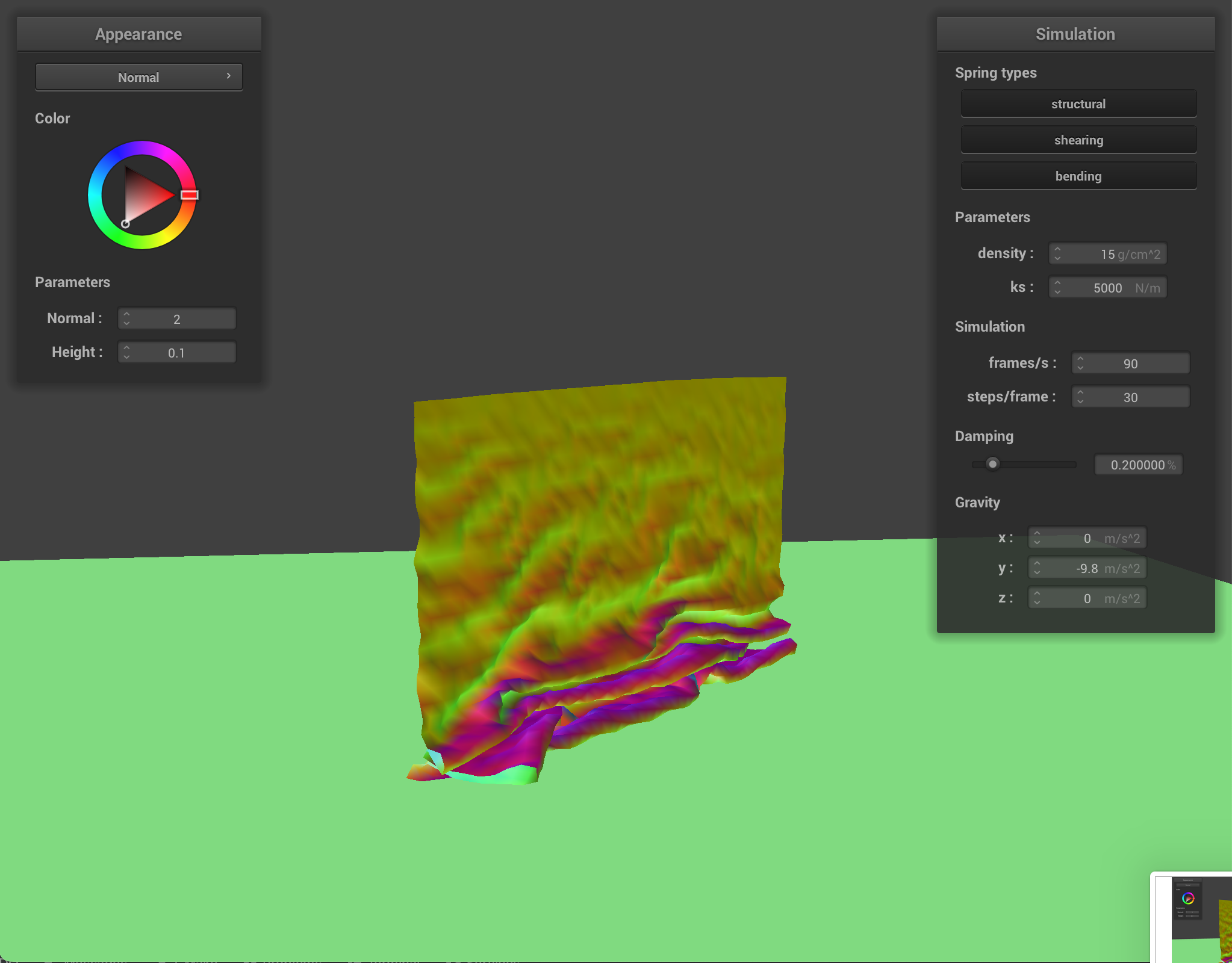
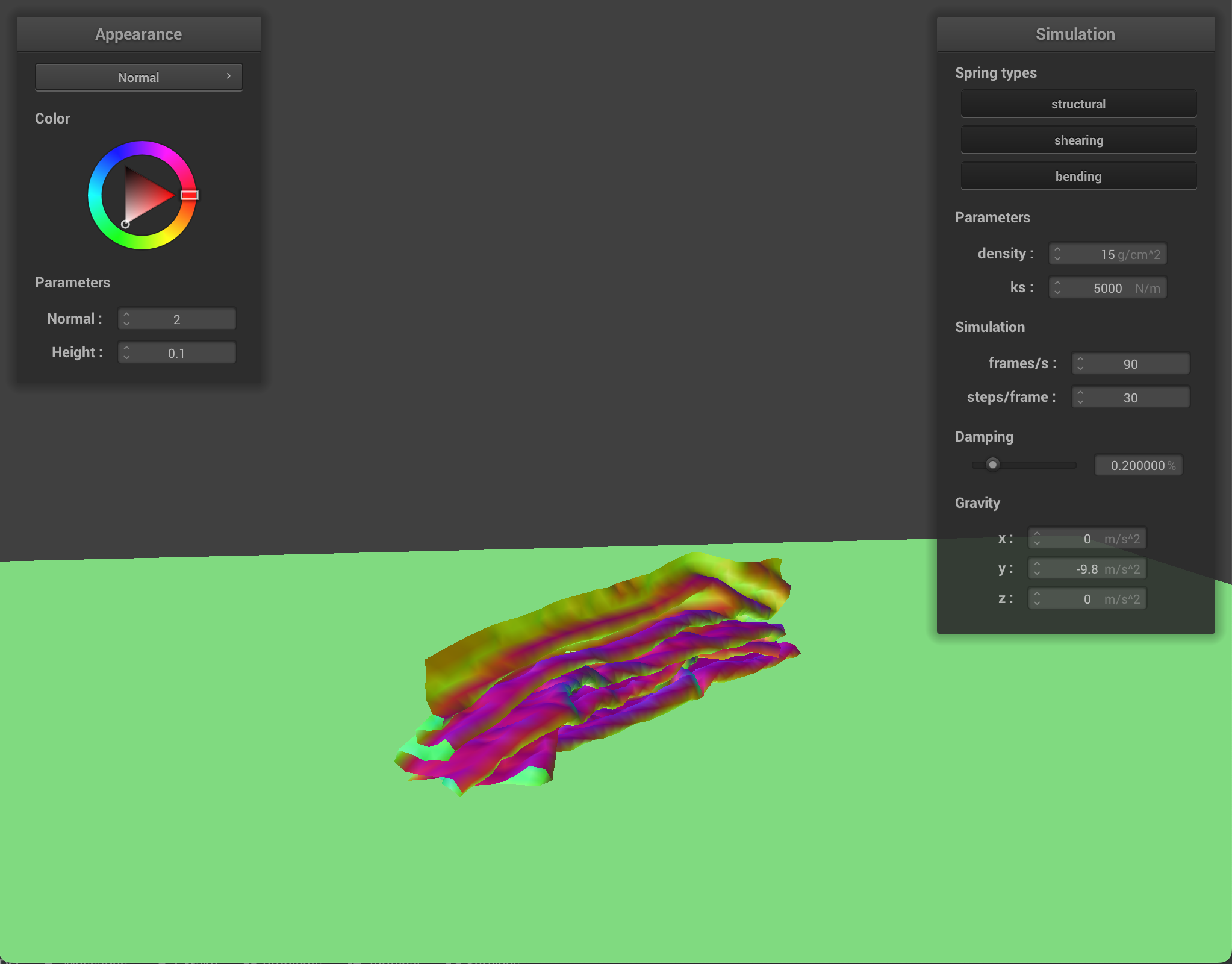
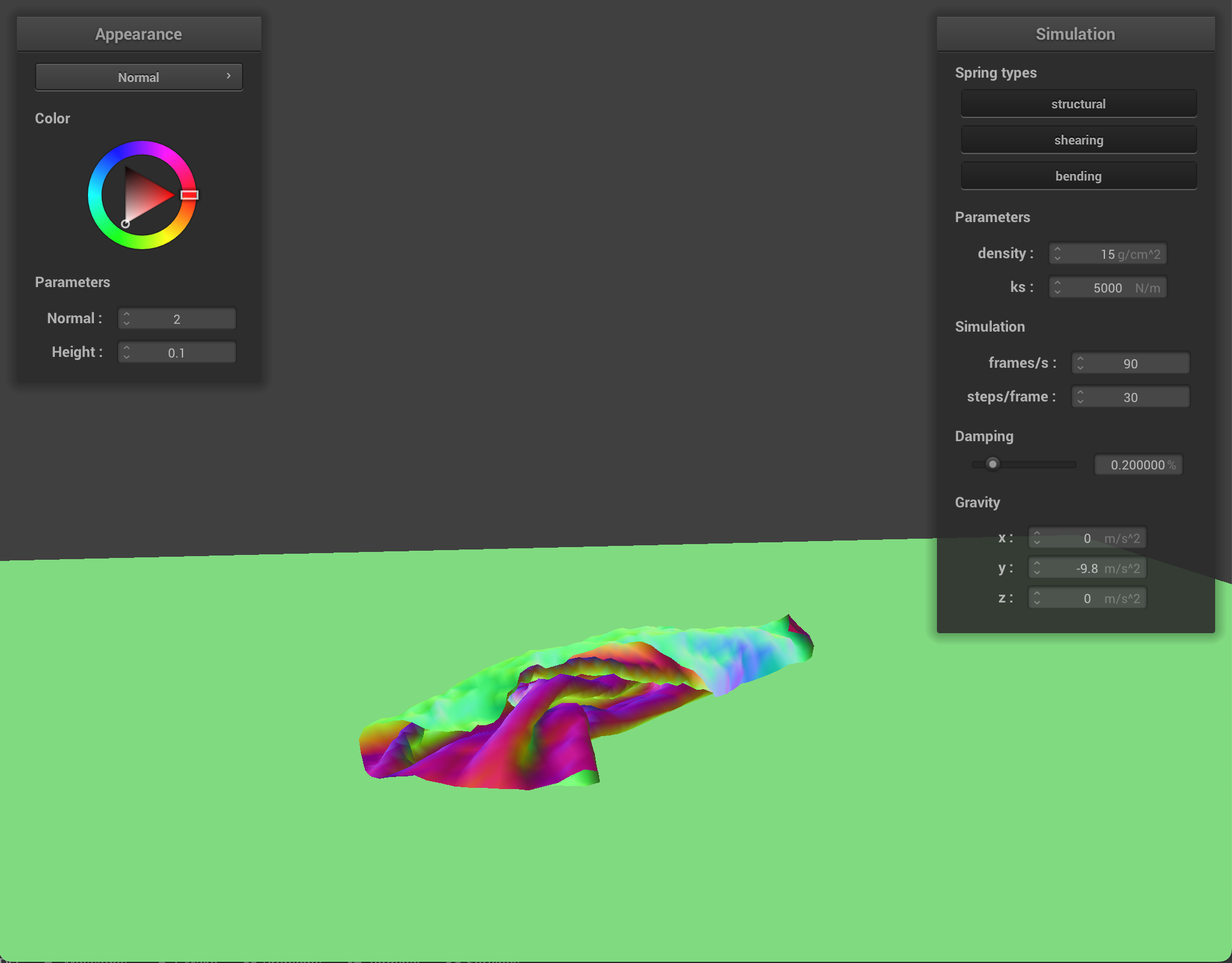
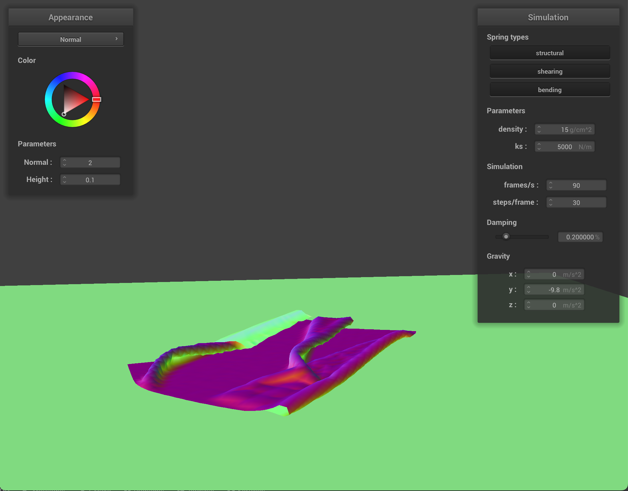
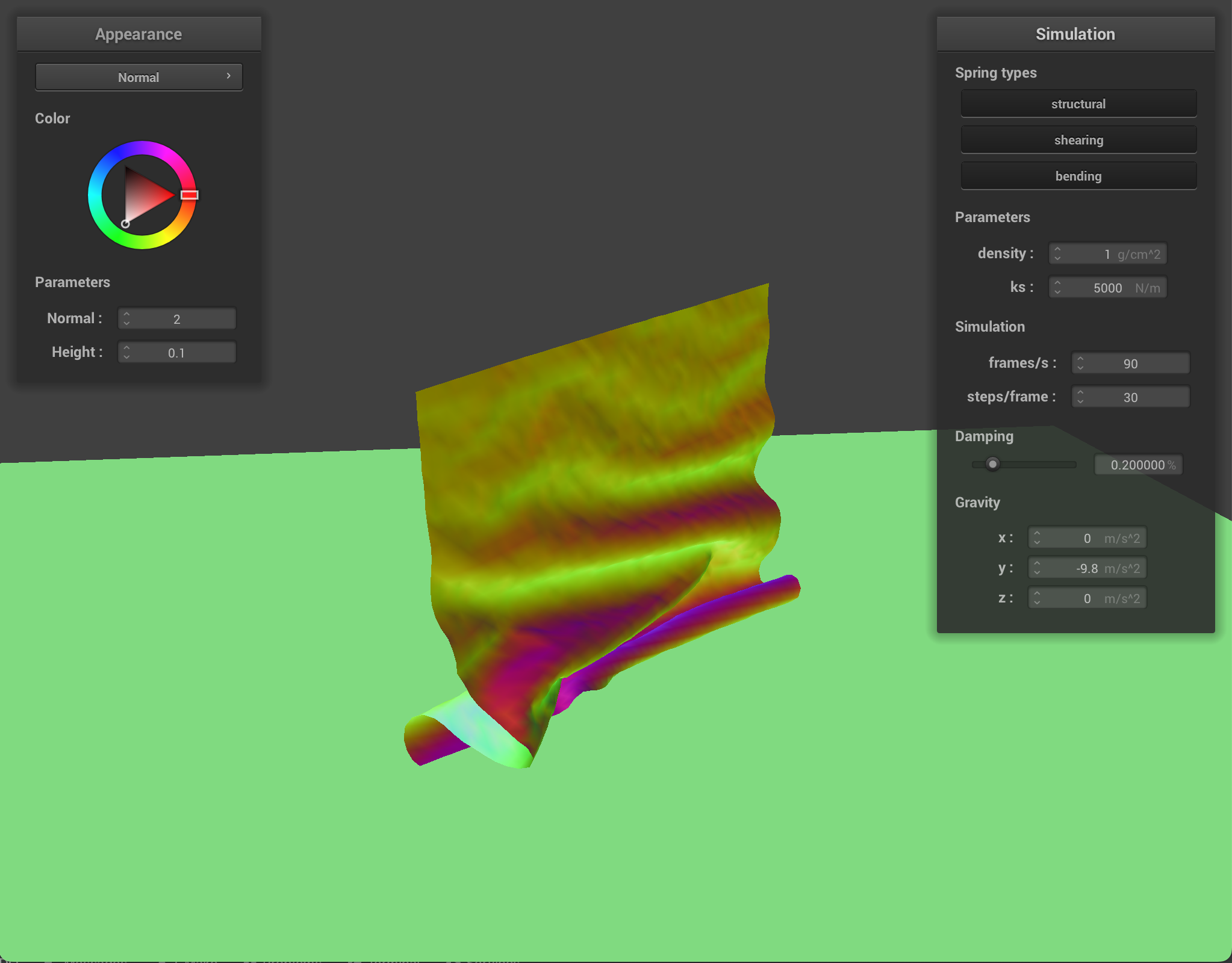
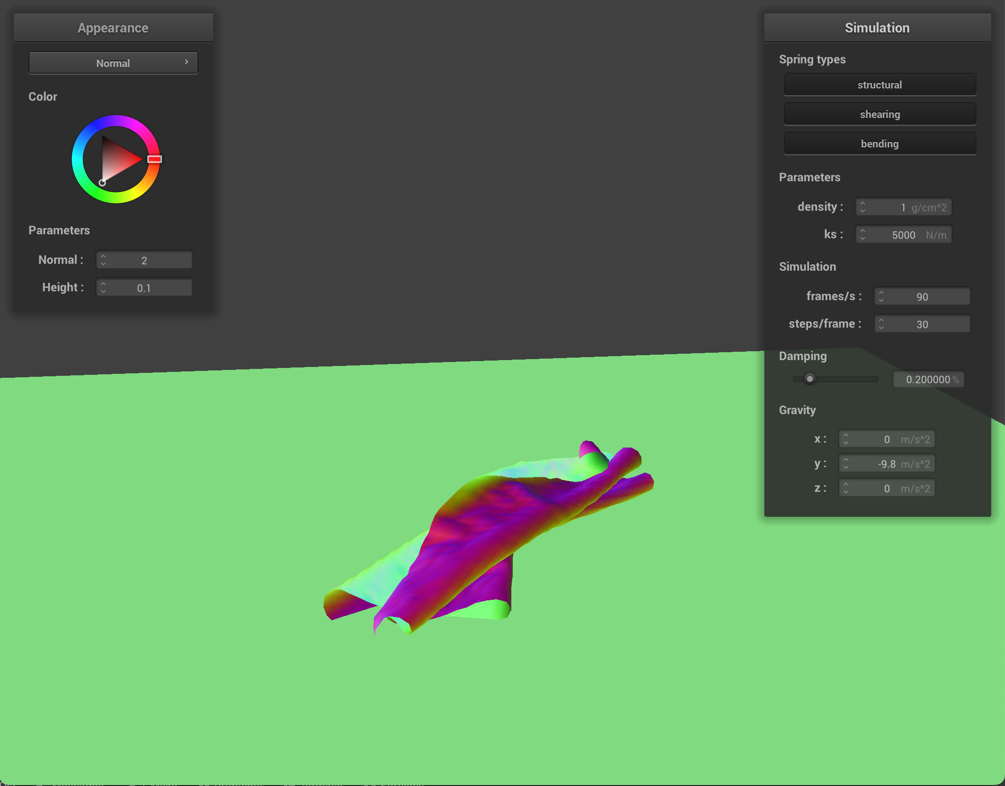
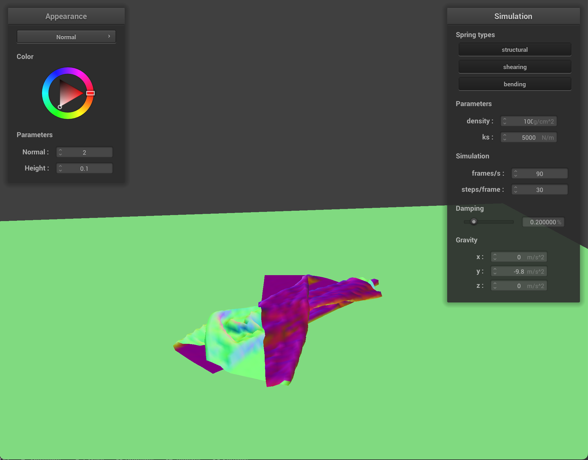
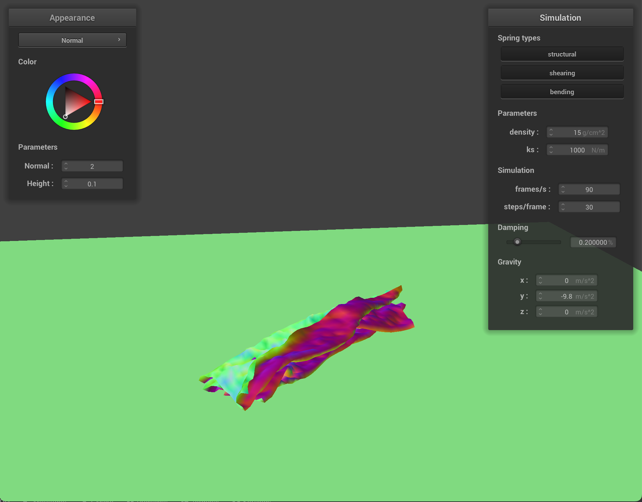
For damping, we experimented with low damping = 0.011494% and high damping = 0.758621%. For both low and high damping, there was no visible difference in the final resting state appearance of the cloth, however, the process to get to the resting state was very noticeable. For low damping, the cloth took an extremely long time (didn’t time it exactly but at least several minutes) to converge to a resting state, while for high damping, the cloth almost immediately came to a resting state. This happens because damping is directly proportional to the amount of energy lost at each time step so low damping means very little energy being lost. The process of the cloth with low damping converging to a final resting state was very interesting (and long!) and below are some screenshots of the process the cloth took to come to a resting state.
|
|
|
|
|
|
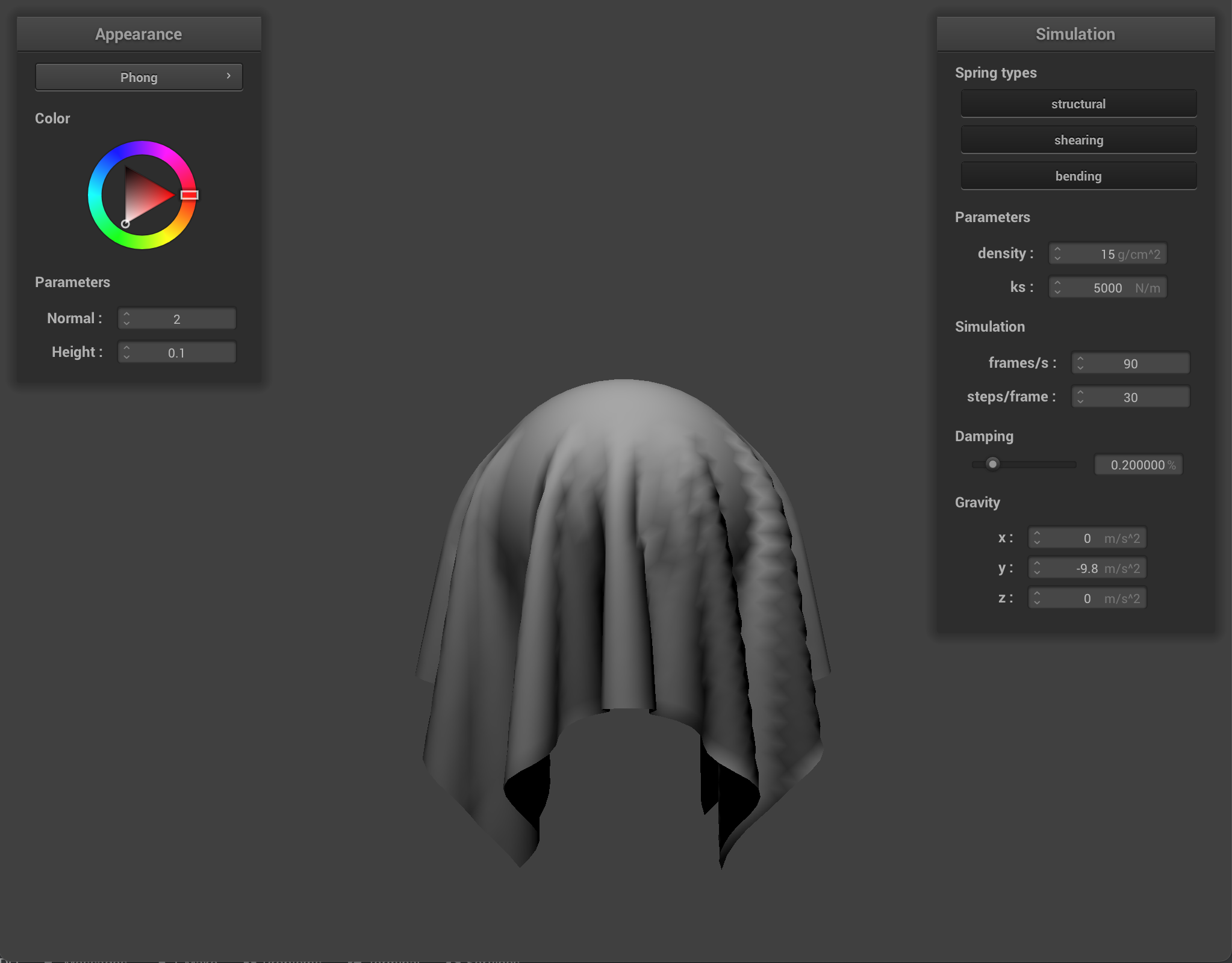
We implement support for cloth collision with spheres and planes. We add support for this in our Cloth::simulate() function by iterating through all the point masses, and for each point mass, we also iterate through all the Collision Objects and check if there are collisions with other primitives. For sphere collision, we first check if the point mass intersects with the sphere or is inside the sphere in Sphere::collide(). We do this by checking the point mass’ position minus the sphere origin and normalizing it and checking to see if this value is less than or equal to the sphere radius. If the point mass does intersect with the sphere or is inside it, we want to bump up our point mass to the surface of the sphere to avoid the cloth going through the sphere instead of draping over the sphere like how cloth is supposed to behave in real life. So next, we calculate the tangent point or where the point mass should have intersected the surface of the sphere. We do this by multiplying the radius of the sphere by the unit vector of the difference between the point mass position and the sphere origin. We then add the origin to extend the path to the surface. Next, we calculate the correction vector to apply to the point mass position by taking the difference of the tangent and point mass’ last position. We can now update the point mass’ new position with the point mass’ last position added to the correction vector which is scaled by 1 - friction. For plane collision, we again start by checking if the point mass is inside the plane or if it crosses over the plane in Plane::collide(). We can check this by taking the dot product of the plane normal and the the difference between the point mass last position and a point on the plane and checking to see if this value is negative, and applying the same check for the point mass’ position. If either of those checks are negative, then we know we need to bump up some positions to avoid the cloth falling through the plane. We first calculate the tangent vector using the ray plane intersection equation from ray tracing, calculating the correction vector by taking the difference of the tangent and the point mass’ last position then adjusting by a small surface offset displacement multiplied by the plane normal. Similar to what we did for the sphere, we then update our point mass’ position.
|
|
|
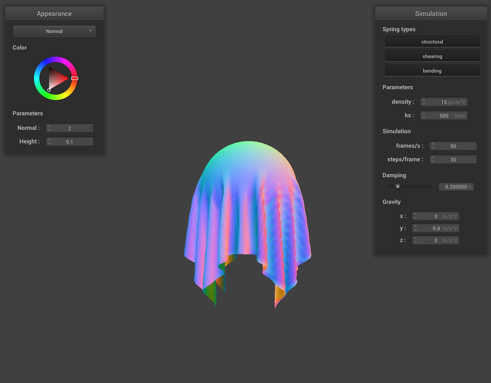
At ks = 5000, if we look close enough, we can tell the object the cloth is covering is a sphere, as the cloth hugs the sphere and appears to have some stiffness in the cloth but not too stiff.
At ks = 500, we can clearly tell the object under the cloth is a sphere because the cloth behaves like stretchy fabric and the folds of the cloth tightly hug the sphere.
At ks = 50000, we can barely tell what object the cloth is draped over as the cloth appears rather stiff and the folds don’t hug the sphere as tightly.
Our results make sense because as we learned in part 2, ks represents the spring constant and is directly proportional to the stiffness of a spring/object. This indicates a higher ks means the cloth is stiffer, while a lower ks makes the cloth more elastic/stretchy.
To ensure that the cloth doesn’t clip when it falls or folds on itself, we add support for self-collision by implementing spatial hashing so that the simulation can run in real-time. At each time step, we build a hash table that maps a float to a vector< PointMass *>, where the float represents a 3D box volume in the scene and the vector< PointMass *> consists of all the point masses within that 3D box volume.
To achieve this, we implement the Cloth::hash_position, which generates a unique key for our hash table, and Cloth::build_spatial_map, which builds the spatial map. To generate a float that represents a specific 3D box volume, our Cloth::hash_position function takes in a point mass position and involves partitioning the 3D space into 3D boxes with dimensions w * h * t, where w = 3 * width / num_width_points, h = 3 * height / num_height_points, and t = max(w, h). Then, using the point mass position, we truncate its coordinates to the closest 3D box. Taking these truncated coordinates, we create a unique float key computing the polynomial x^3 + y^2 + z. To build the spatial map, Cloth::build_spatial_map loops through all the point masses and generates a key using the point mass position using Cloth::hash_position. Then, we check if an element with that key exists within the map. If no element exists, we create a new entry in the map, where key maps to a new vector< PointMass *>. Then, (regardless of whether an element exists for this key or not) we push back this point mass into the vector< PointMass *> at pointed to by map[key].
After building the map, we implement Cloth::self_collide, where we loop through the point masses, look up the point mass in the hash table to find other point masses that share the same 3D volume, and then adjust the point mass position if it is too close to another point mass in the 3D volume. More specifically, a pair of point masses are too close if they are within 2 * thickness apart in distance. If this is the case, we compute a correction vector that can be applied to the point mass such it is 2∗thickness distance apart from the other point mass. The final correction vector to be applied to the point mass's position is the average of all of these pairwise correction vectors scaled down by simulation_steps.
Once these functions have been implemented, we incorporate self-collision into the simulation by calling Cloth::build_spatial_map in Cloth::simulate, then loop through all the point masses and call Cloth::self_collide on each point mass.
|
|
|
|
|
|
density as well as ks and describe with words and screenshots how they affect the behavior of the cloth as it falls on itself.
|
|
|
|
Cloth at density = 1 |
||
|

|
|
|
Cloth at density = 100 |
||
|
|
|
|
Cloth at ks = 1,000 |
||
|
|
|
|
Cloth at ks = 10,000 |
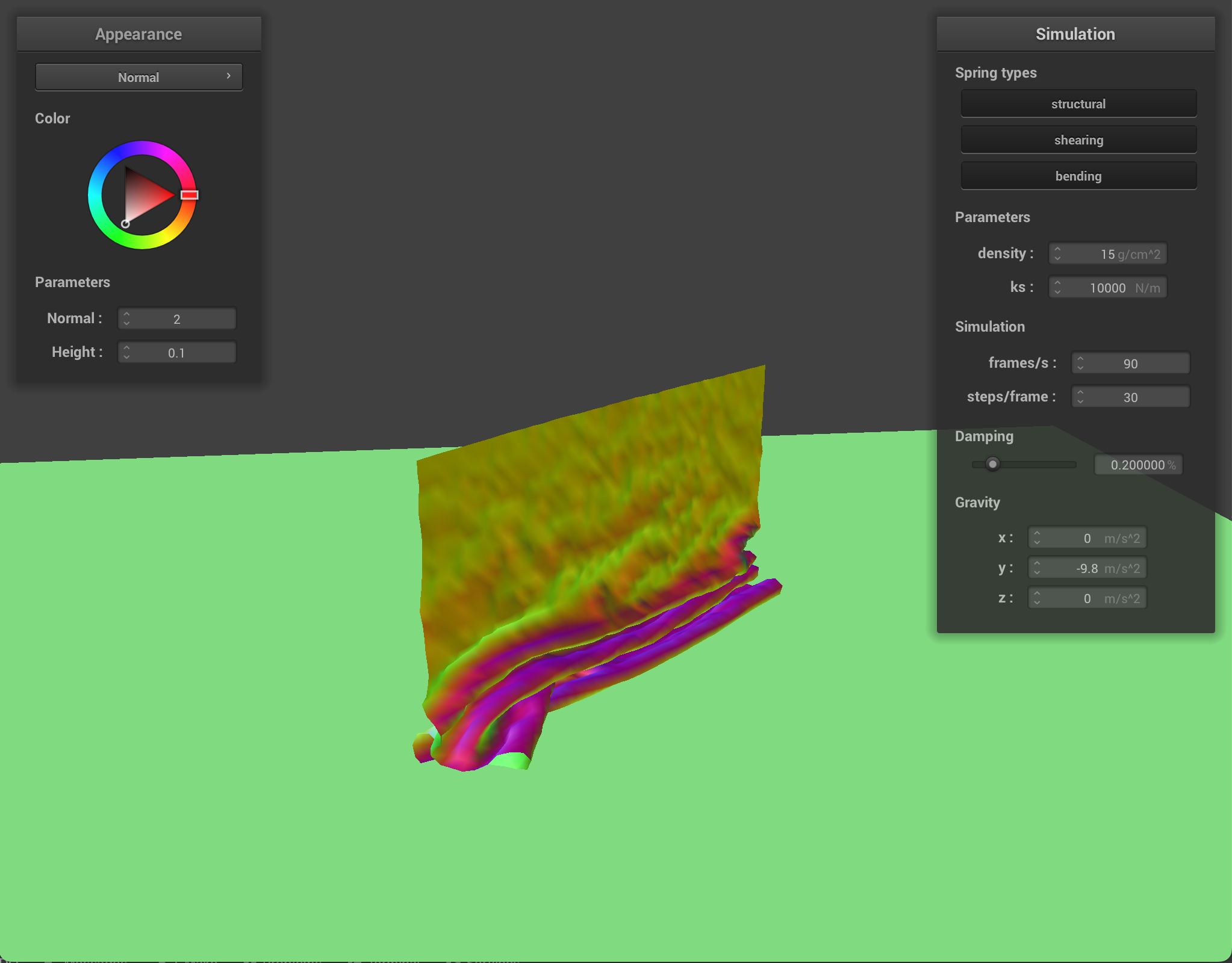
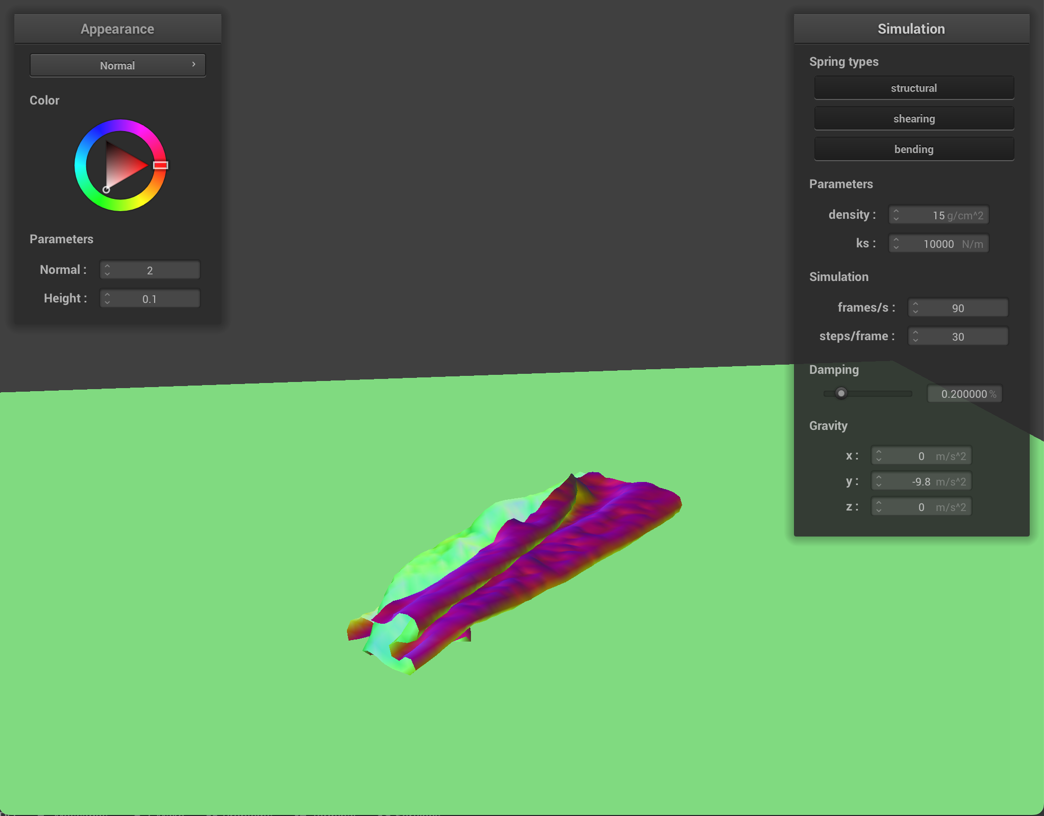
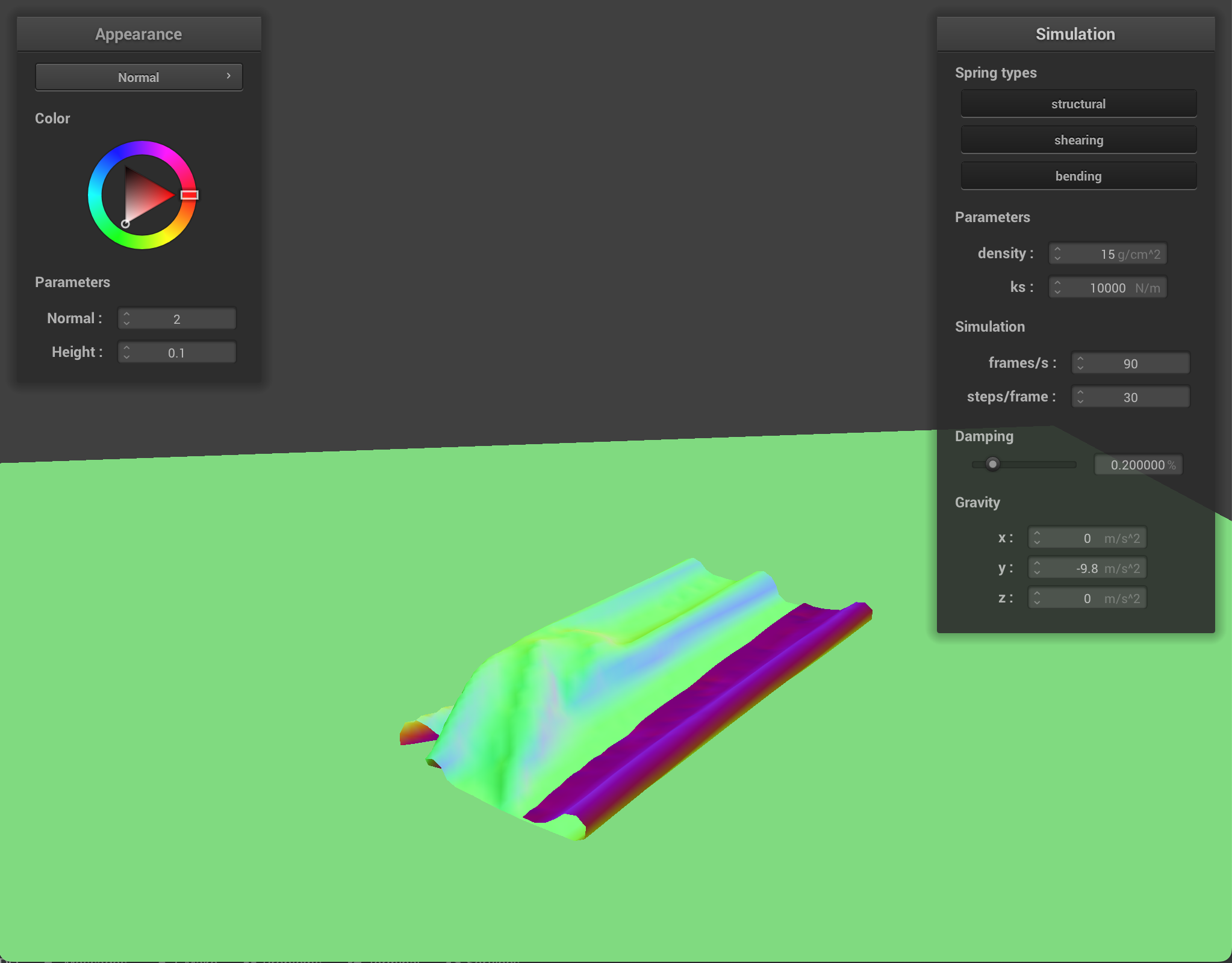
At low-value density, the cloth has no small wrinkles and the cloth folds over very smoothly in large bends. At higher density, the cloth has more wrinkles and has many small folds. With lower spring constant values, the cloth shows more wrinkles and appears very elastic and bouncy. With higher spring constant values, the cloth feels more rigid and does not have as many folds or show as many bounces when falling.
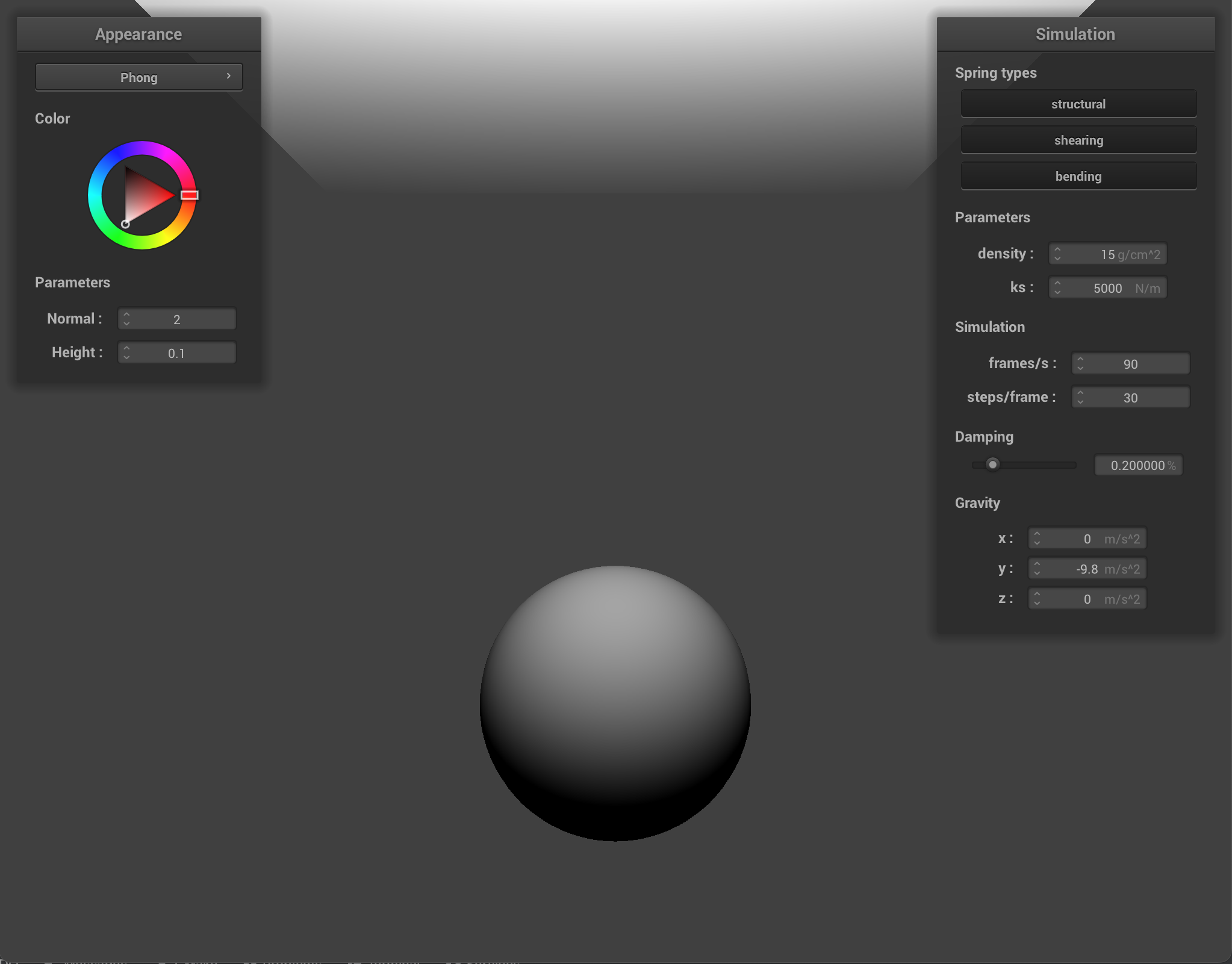
We now implement the following in GLSL: diffuse shading, Blinn-Phong shading, texture mapping, displacement and bump mapping, and environment-mapped reflections.
For diffuse shading, we use the Lambertian shading formula:
where we output the color of the fragment to be the diffusely reflected light.
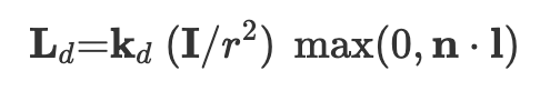
We implement the Blinn-Phong shading model using the equation:

where r is the distance from the vertex to the light source, n is the surface normal, l is the vector from the vertex to the light source, h is the bisector or halfway vector between the viewpoint and light source vectors, and I is the intensity of light.
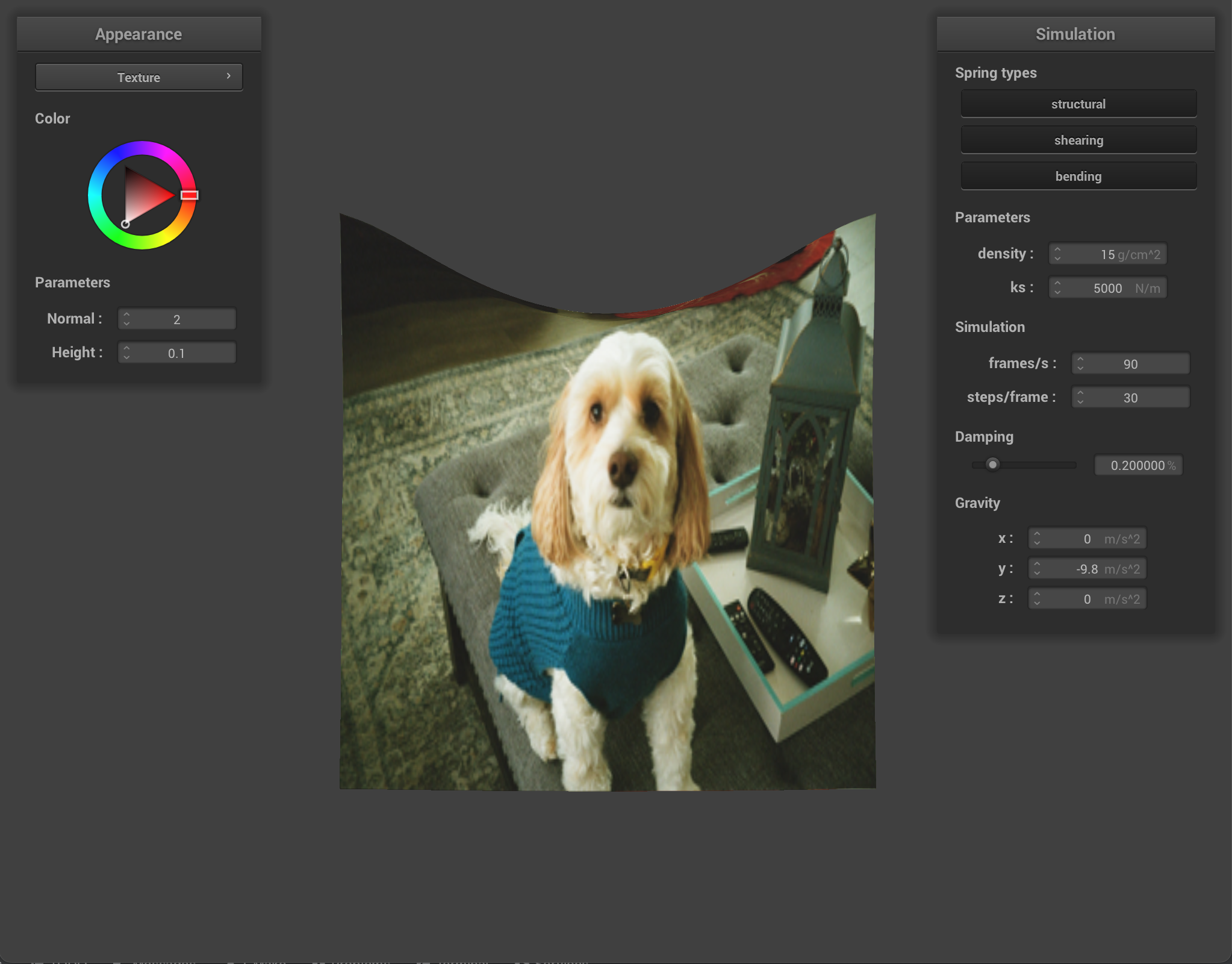
For texture mapping, we are given a v_uv coordinate to use in the fragment shader, and we use the built-in function texture() to sample from the texture u_texture_1 uniform at the texture space coordinate v_uv. We return this sample as the color of the fragment.
For bump mapping, we compute the local space normals by looking at how the height changes as we make small changes in texture coordinates u or v. We do this using the following system of equations:
where h(u,v) is a function that returns the height encoded by a height map at u and v, w and h are the width and height of our texture, and k_h and k_n are the height scaling factor and the normal scaling factor represented in our shader. The local space normal is n_o = (-dU, -dV, 1), and our displaced model space normal is n_d = TBN * n_o, where TBN is a matrix consisting of the original model-space normal vector, the tangent vector, and the bitangent vector. We then update the normals within our Phong shader implementation to be n_d.
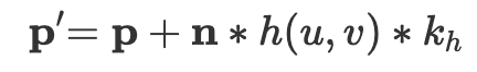
Displacement mapping expands upon bump mapping, where in addition to computing the local space normals, we also update the positions of vertices. To do this, we displace the vertex positions in the direction of the original model space vertex normal scaled by the normal scaling factor:
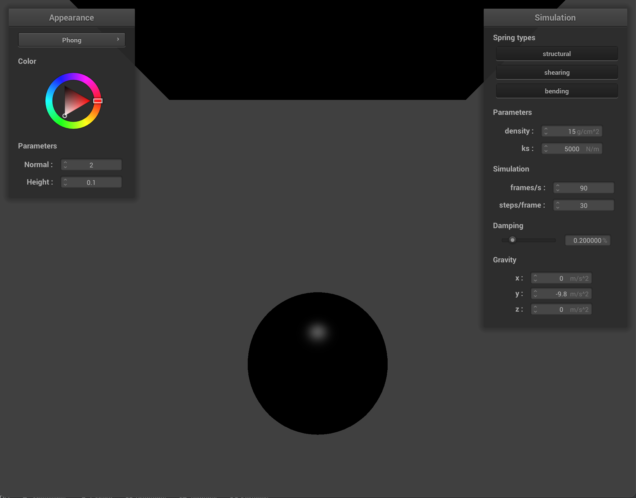
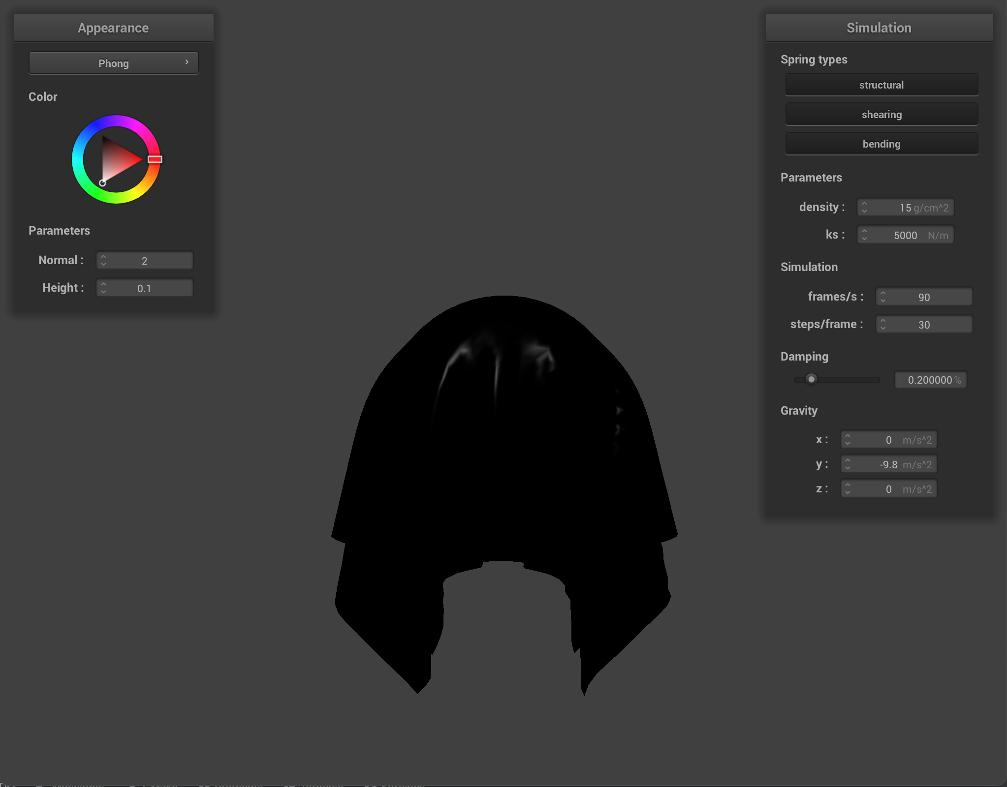
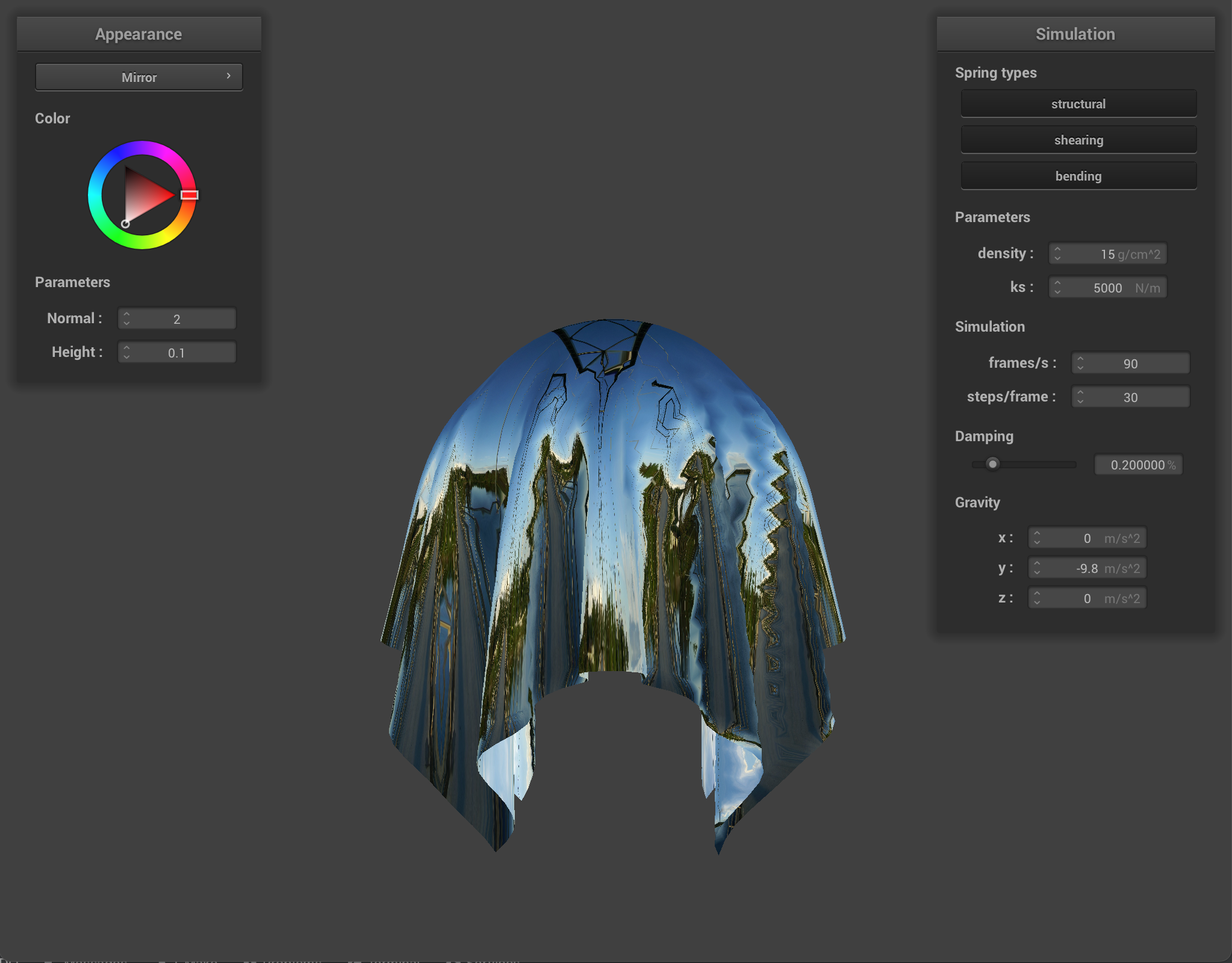
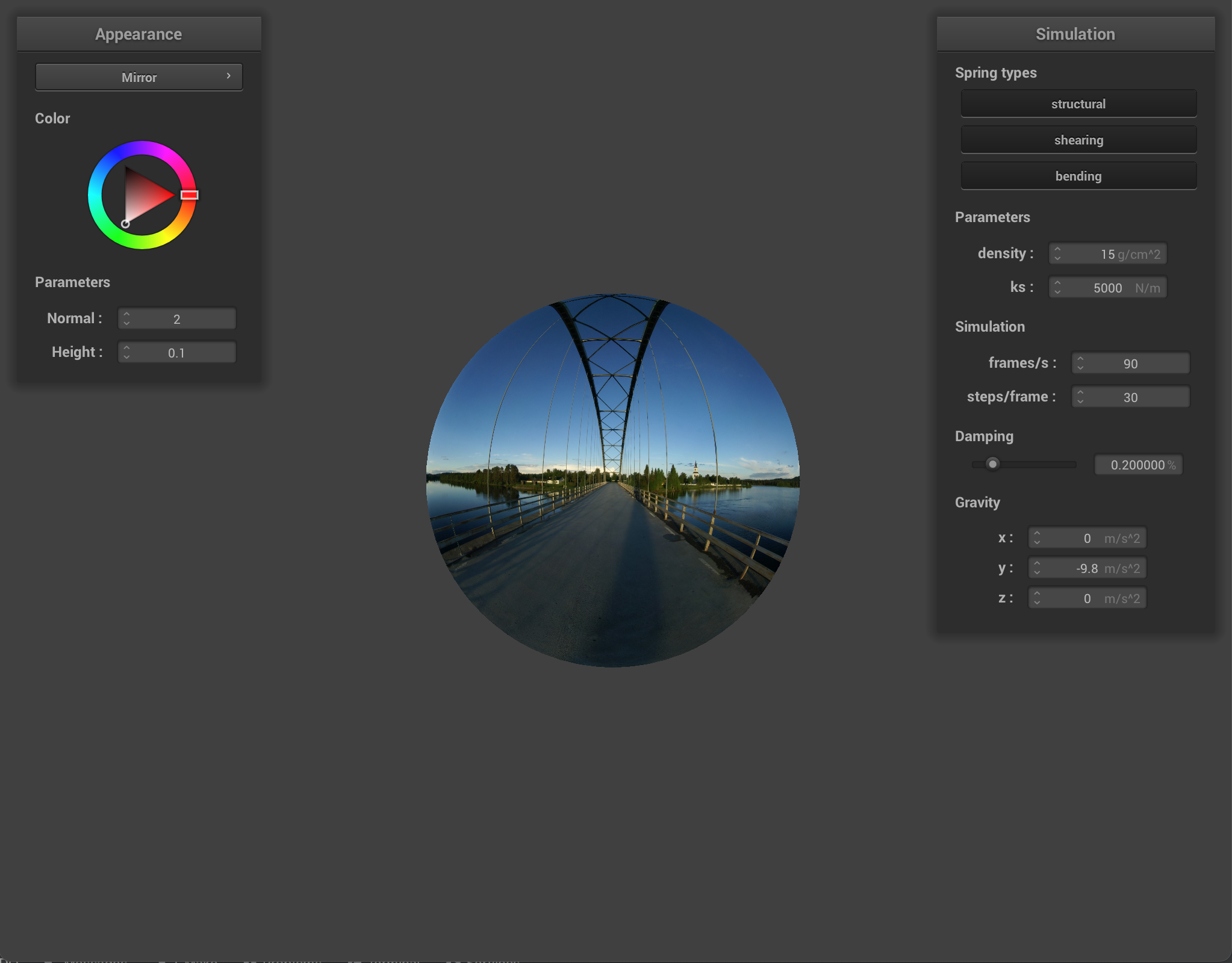
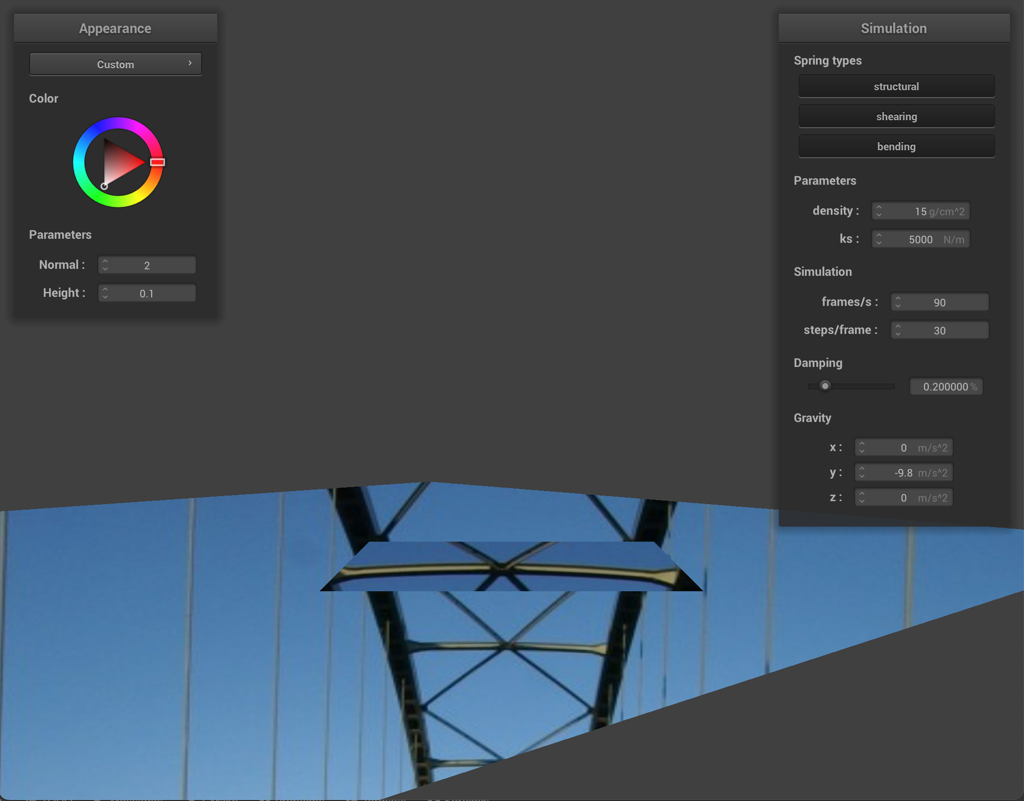
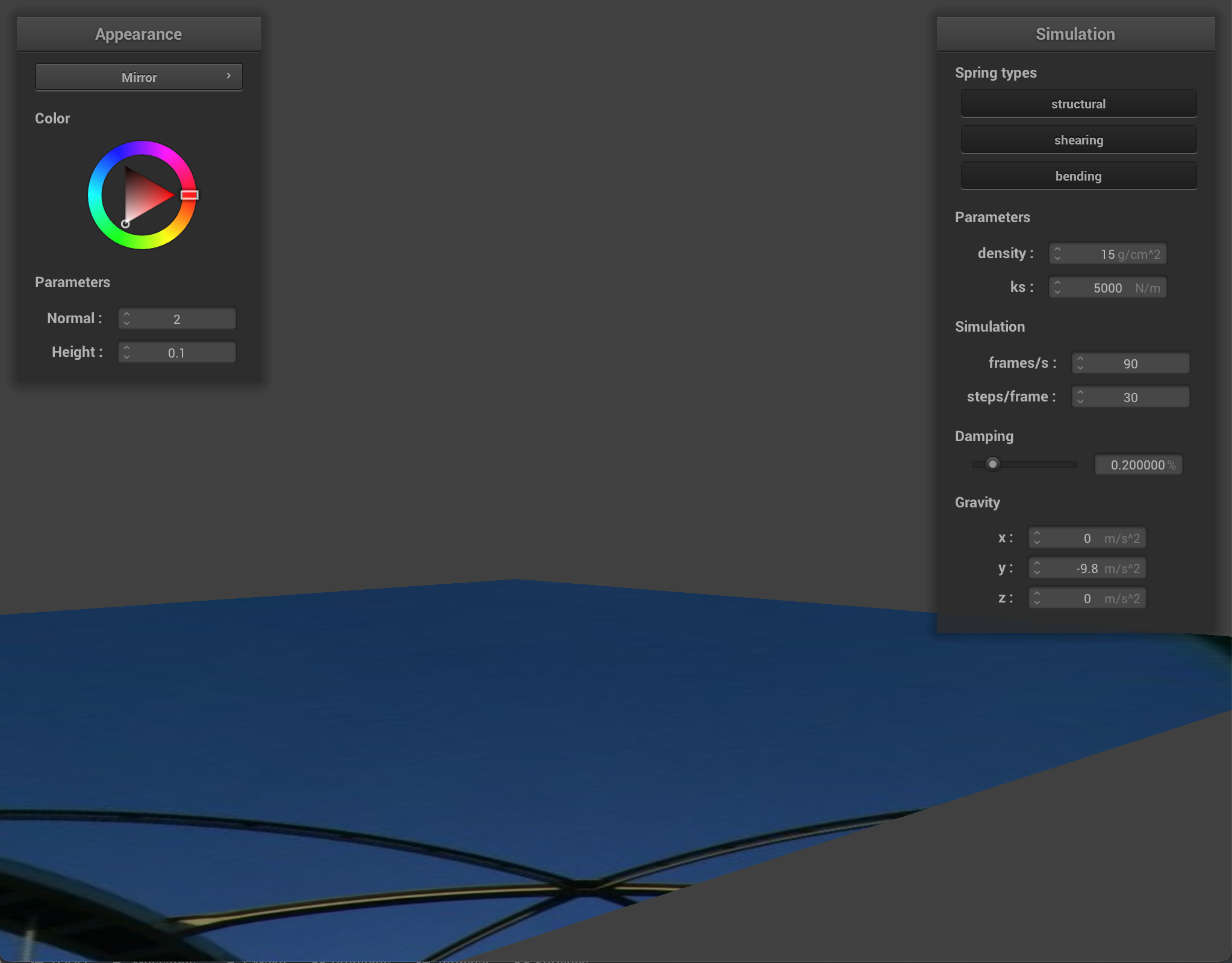
Lastly, for environment-mapped reflections, we simulate a mirror-like material using a given cubemap texture. We do this by computing the outgoing eye ray from the camera’s position and fragment’s position, then reflecting it across the provided surface normal to get the incoming direction. Lastly, we sample environment cubemap at the incoming direction before returning it.
Shader programs are important to the graphics pipeline; they are programs that run in parallel on GPU, outputting a single 4-dimensional vector representing the color at a particular input point. The shaders we implement are written in GLSL and consists of vertex shaders and fragment shaders. Vertex shaders apply transformations to properties of vertices such as position and normal vectors. Fragment shaders process fragments, which are created after rasterization; these shaders take the geometric attributes of the fragment and compute a final color value.
Expanding upon before, the Blinn-Phong shading equation is the sum of three components: an ambient light component, a diffuse component, and a specular reflection component.
|
|
|
|
|
|
|
|
|
pinned2.json |
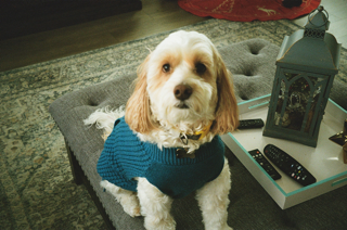
texture_2.png.
|
|
|
|
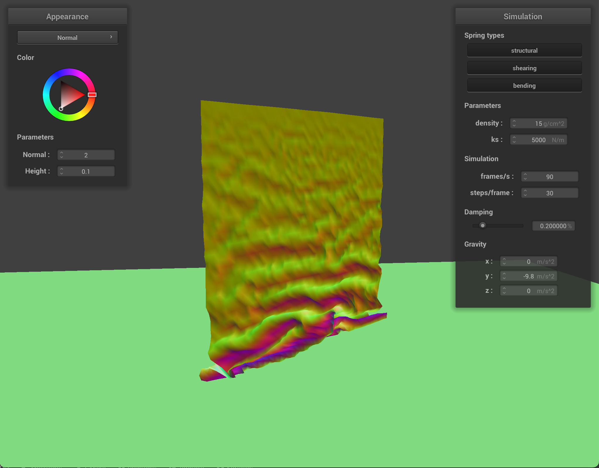
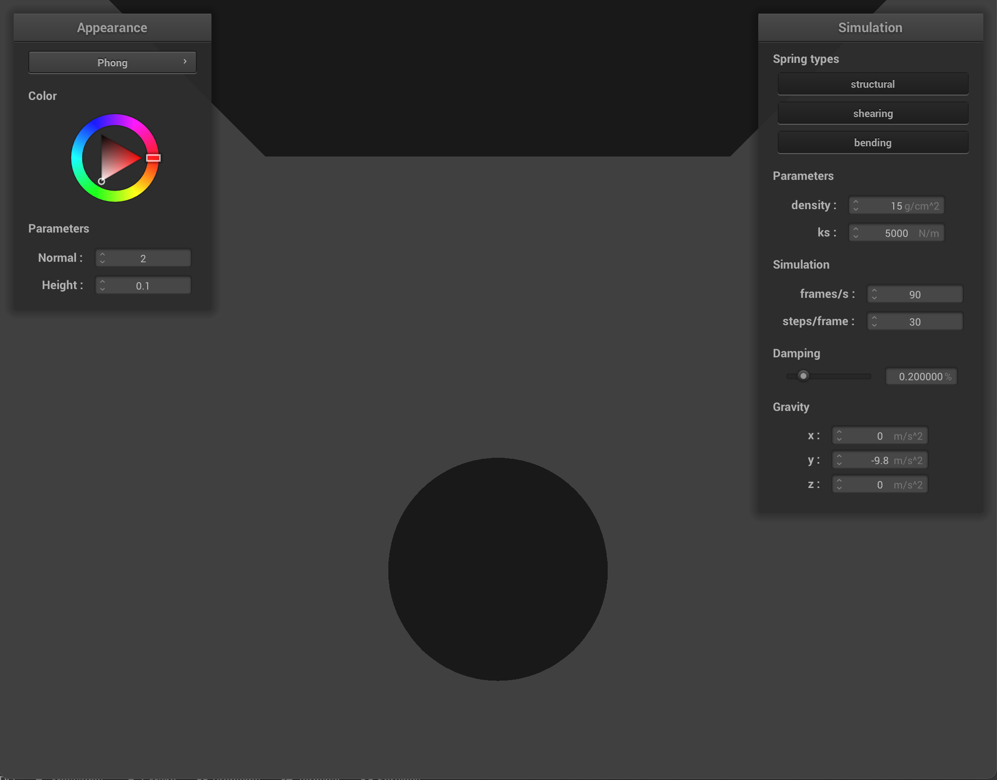
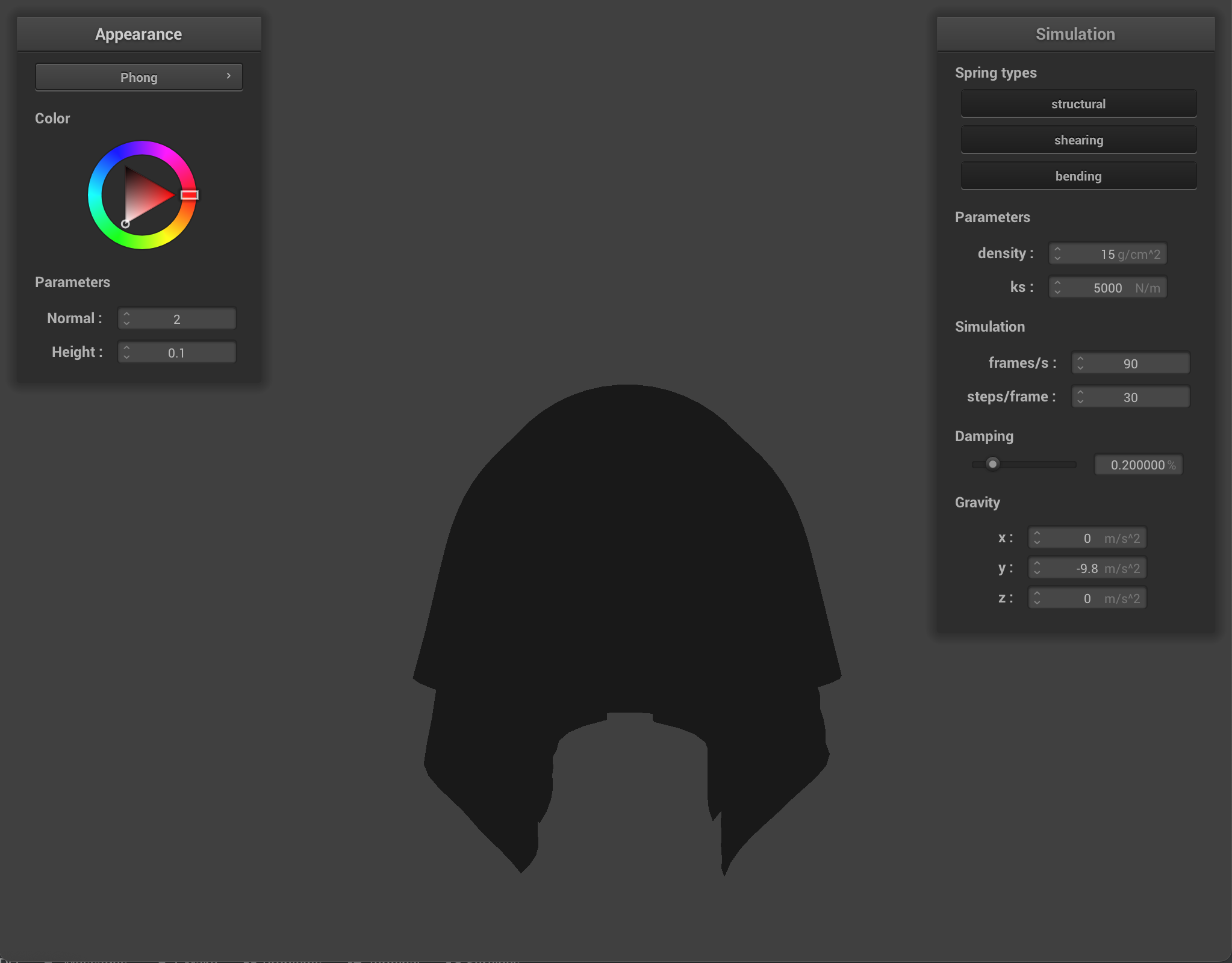
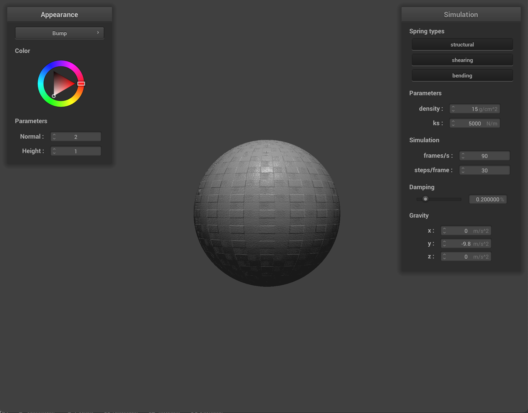
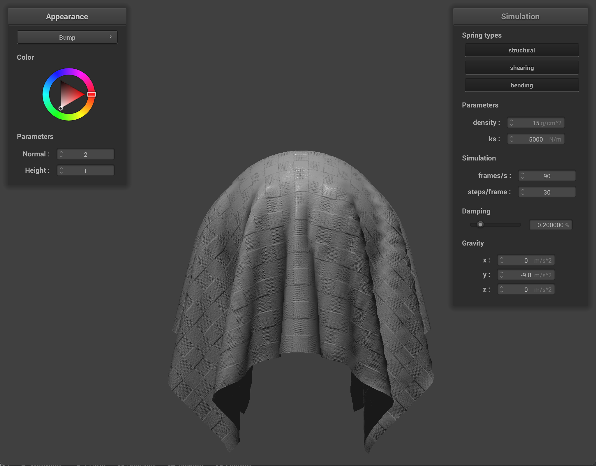
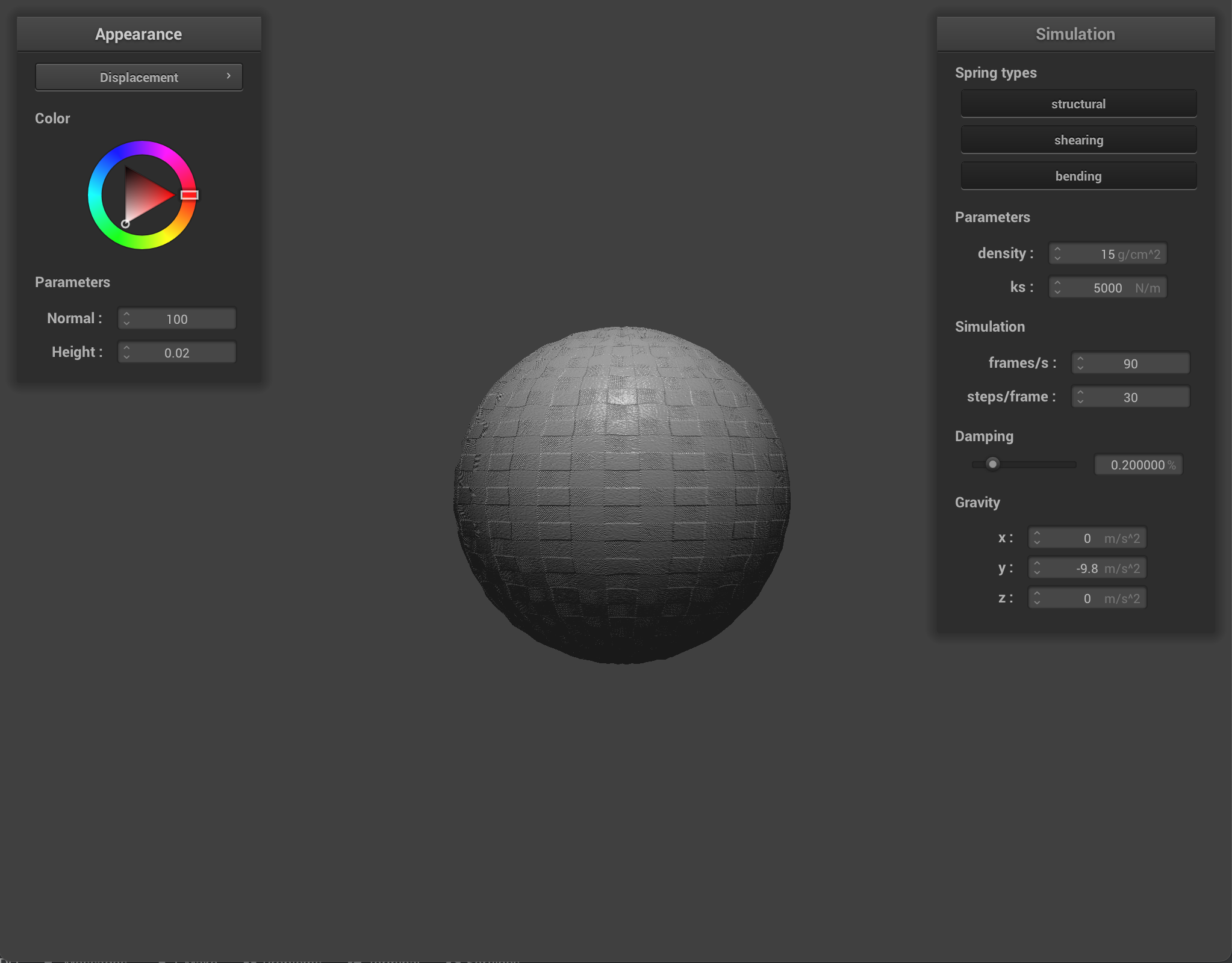
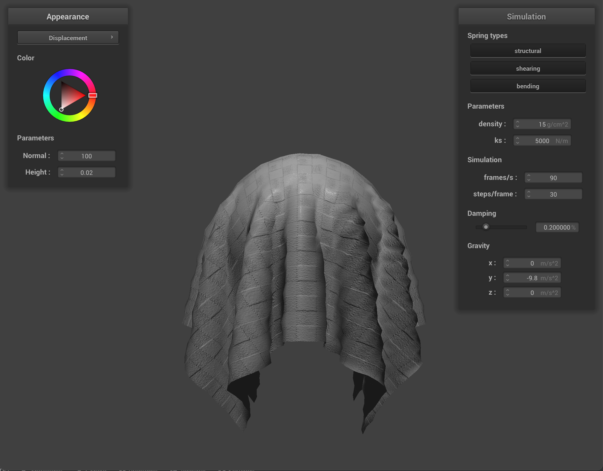
Bump mapping involves modifying the normal vectors of an object so that the fragment shader can apply illusionary details, such as bumps, to the cloth, however when applied, the bump map does not apply to change the geometry or appearance of the object. Displacement mapping also involves adjusting the normal vectors, but it also requires modifying the position of vertices, so the displacement map, as seen above, does change an object’s appearance, as seen especially within the cloth, which appears more groovy.
-o 16 -a 16 and then -o 128 -a 128.
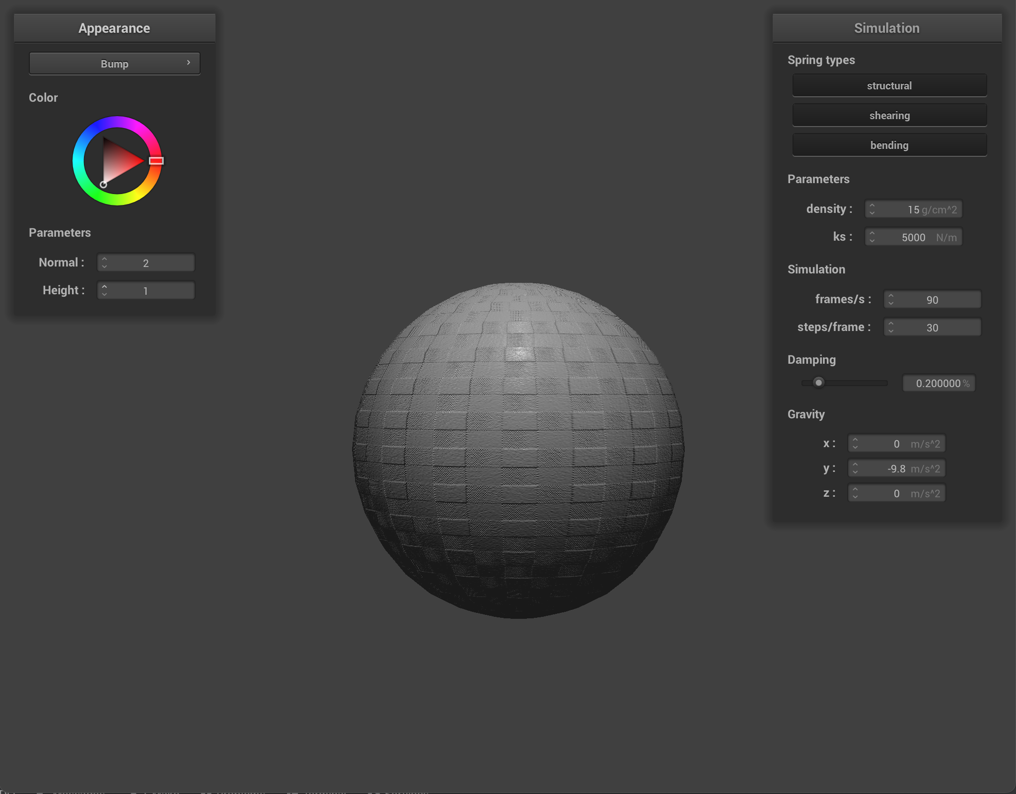
-o 16 -a 16 |
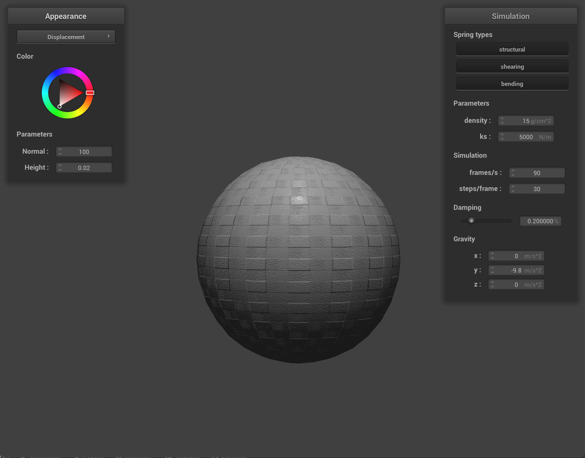
-o 16 -a 16 |
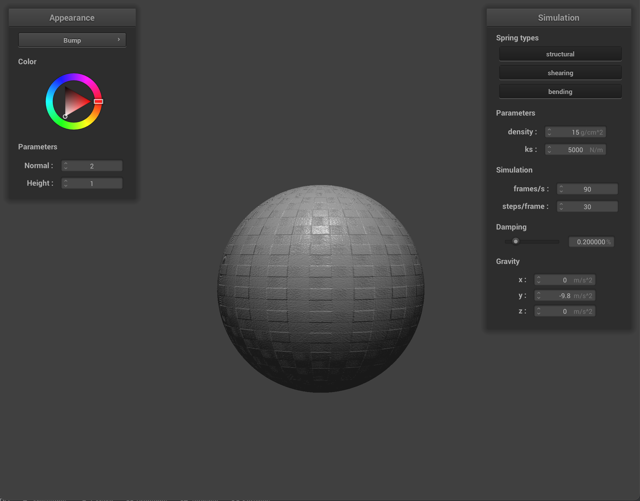
-o 128 -a 128 |
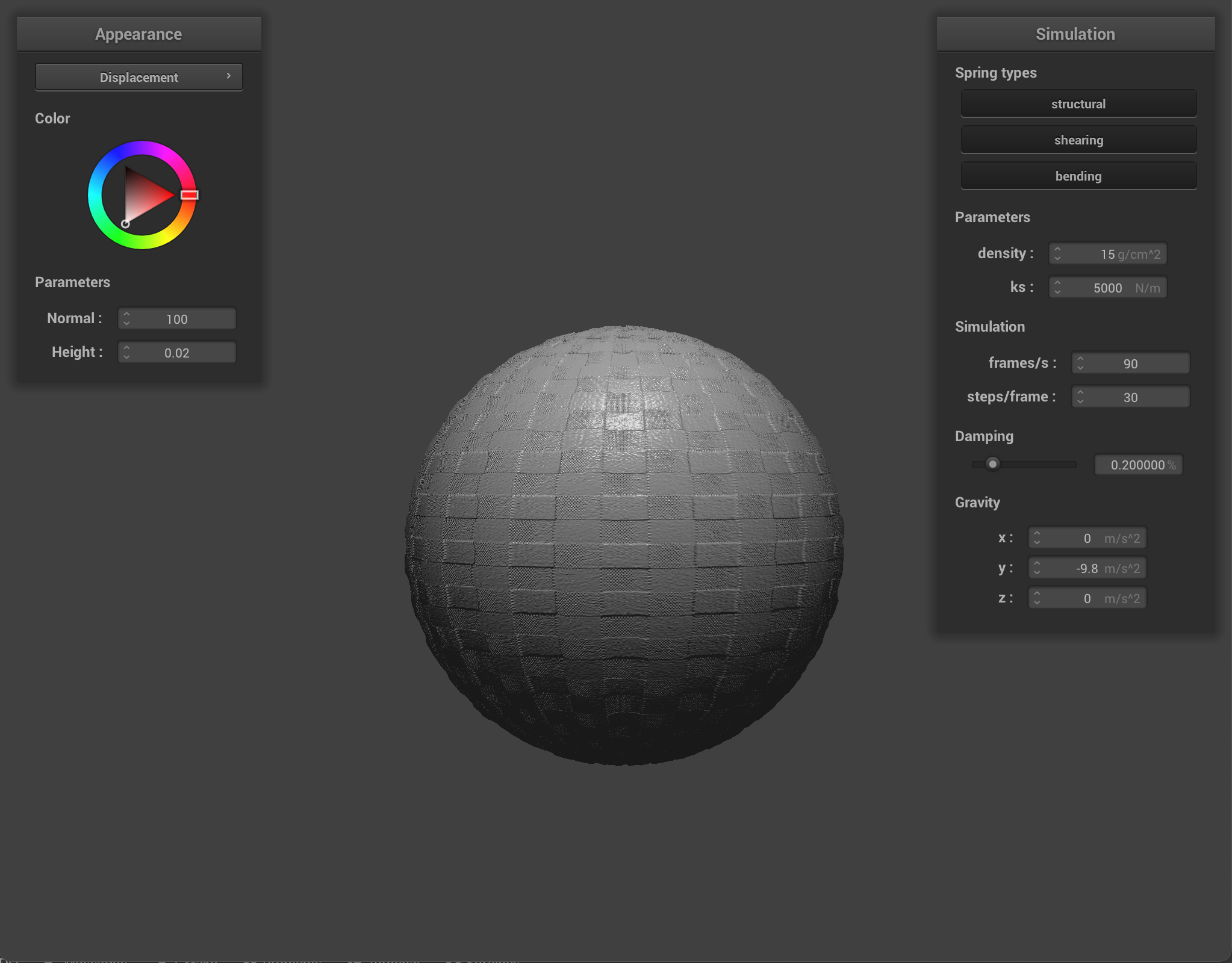
-o 128 -a 128 |
At the low resolution of 16x16, there seems to be virtually no difference between the two spheres when using the bump shader and displacement shader. At a higher resolution of 128x128, on closer look, the edges are slightly sharper when performing displacement mapping on the sphere.
|
|
plane.json |
plane.json, for comparison |
For our custom shader, we modified our mirror shader! Instead of reflecting the incoming eye-ray across the surface normal to get the outgoing direction, we instead refracted it with a refraction index of 0.33 (the refraction index from water to air).