CS 184: Computer Graphics and Imaging, Spring 2023

Project 3-1: Path Tracer

Annie Lin, Vivian Liu

Website URL: https://cal-cs184-student.github.io/proj-webpage-photoreceptor/proj3-1/index.html

Overview

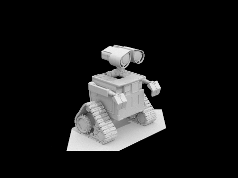
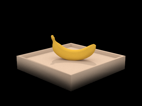
In this project, we implemented a renderer capable of generating realistic images using a pathtracing algorithm. We first implemented ray generation and scene intersection, which included translating coordinates from image space to camera space, generating pixel samples, implementing intersection tests between rays and triangles, and implementing intersection tests between rays and spheres. We learned here that even with normal shading, our renders all took a very long time to render, even for .dae files that weren’t as complex, so for the next part, we implemented bounding volume hierarchy to speed up the rendering times of our .dae files. This included constructing the BVH itself (which is essentially a binary tree) and which required us to figure out how to split primitives into left and right nodes recursively. We decided to sort primitives by arbitrarily choosing a heuristic where we split primitives based on whether they were less than the average of centroids along the greatest axis (sorted on the left if yes, and split to the right if not). We also implemented intersection tests with the bounding boxes and intersection tests with the BVH, both of which would significantly speed up our rendering times on files with normal shading as we could filter out which rays to consider when rendering. We then implemented direct illumination which included implementing a diffuse BSDF (Bidirectional Scattering Distribution Function), zero-bounce illumination which is light that reaches the camera but doesn’t bounce, and direct lighting with uniform hemisphere sampling and by importance sampling lights. We also implemented global illumination, which makes our renders of diffuse BSDFs even smoother, using recursion to estimate how much light arrives at a point and Russian Roulette for an unbiased random termination method. Finally, we implemented adaptive sampling, which reduces noise even more in our renders (but the tradeoff is longer render times) by using a fixed number of samples per pixel and by concentrating samples in certain parts of an image that require more samples for proper rendering. After this project, we now have a working renderer that can render realistic images with .dae files. We also have a better understanding of what goes behind the scene when we see hyperrealistic rendered images in the real world.

Part 1: Ray Generation and Scene Intersection (20 Points)

Walk through the ray generation and primitive intersection parts of the rendering pipeline.

For ray generation, we went through a series of steps: first, we transform image coordinates to camera space, second, we then generate the ray in camera space, and third, we transform the ray into world space. We performed the first step by calculating/drawing out how image coordinates would translate to the camera space. We converted hFov and vFov to their radian forms, and since we are given the Vector3D camera origin (pos), we just need to figure out how to calculate the Vector3D of the camera direction. We realized that the width and height of the sensor is 2*tan(0.5*hFov) and 2*tan(0.5*vFov) respectively. We then realized we can calculate the x direction of the camera by subtracting by 0.5 and multiplying by the width, and similarly subtract y by 0.5 and multiplying by the height for the y direction. We now have the camera direction and so we can now generate the ray in camera space and set the min_t and max_t to nClip and fClip respectively. Finally, we can transform the ray to world space by multiplying the ray’s direction by the camera-to-world rotation matrix and normalize the direction. We don’t have to transform the ray’s origin however because it is already in world space.

For the primitive instruction parts of the rendering pipeline, we implement raytrace_pixel(), where we looped through ns_aa total samples using a for loop and kept track of the running total Vector3D for averaging later. In each iteration of the for loop, we get a Vector 2D random sample using gridSampler->get_sample() which draws a random from a uniform distribution on a unit square. We then add the corresponding values indexed at 0 and 1 of the Vector2D random sample to x and y, our input pixel coordinates, and we then normalize the input coordinates by the width and height of the image which we did by dividing by sampleBuffer.w and sampleBuffer.h respectively. We take these new x and y coordinates to generate a ray using camera->generate_ray() and pass in the resulting ray to est_radiance_global_illumination, which estimates the scene radiance along the ray. We then add the resulting Vector3D to our running total tracker and repeat for the next loop. At the end, we divide the Vector3D running total by ns_aa (our total number of samples), and update the sampleBuffer at the resulting Vector3D, which represents the integral of radiance over the pixel at (x, y).

Explain the triangle intersection algorithm you implemented in your own words.

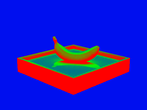
We used the Möller-Trumbore Algorithm and barycentric coordinates to implement our ray triangle intersection. In has_intersection(), we calculated the resulting t, b1, and b2 values using the Möller-Trumbore Algorithm, which used the Vector3D points of the triangle and the corresponding Vector3D normals, as well as the ray’s origin and the ray’s direction. The result was that we had t, beta (b1), and gamma(b2), and we could calculate alpha by doing 1-beta-gamma. We then performed a three line test to ensure each of the resulting barycentric coordinates were >= 0. We then check if our resulting t value is >= the ray’s min_t and similar if t is <= the ray’s max_t. If this is the case, we can then update the max_t of the ray to the value of t and return true. Similarly, for intersect(), we perform Möller-Trumbore to get the resulting vector and barycentric coordinates. We do the three line test and check if t is contained within r.min_t and r.max_t, but this time, we also update corresponding values in isect, our pointer to an Intersection. We assign isect->t, or the t-value of the input ray where the intersection occurs, to the t in our resulting vector (final[0], where final is the result vector containing t and our barycentric coordinates). We assign and calculate the surface normal at the intersection (isect->n) to the calculated surface normal as alpha*n1+beta*n2+gamma*n3 and normalize. We also assign the Intersection’s primitive to the this pointer (the primitive that was intersected), the Intersection’s BDSF to get_bsdf() and update the ray’s max_t value to the resulting t value.

Show images with normal shading for a few small .dae files.

Part 2: Bounding Volume Hierarchy (20 Points)

Walk through your BVH construction algorithm. Explain the heuristic you chose for picking the splitting point.

We first declare a bounding box variable and computed the bounding box of a list of primitives using a for loop which began at start and stopped at end. Inside the loop, we retrieve each primitive pointer, dereference it, and get the associated bounding box using get_bbox(). Using the bounding box we declared outside the loop, we expand() on it by passing in the bounding box of the current primitive. The heuristic we chose for picking the splitting point is the average of centroids along the axis with the greatest bounding box extent. To that end, we also have a counter for the total number of primitives inside the for loop and keep a running total of the sum of all the centroids associated with each primitive’s bounding box. Outside the loop, we calculate the average of the centroids along each axis (x, y, and z). We then initialize a new BVHNode with the bounding box we just created. We then check if the size of primitives we just iterated over is <= max_leaf_size, and if true, we set node->start to start, node->end to end, and return our node because we know that the node we just created is a leaf node. This if case will also serve as our base case for our recursion. If the size is not <= max_leaf_size, we know the node is not a leaf node and that there is more work to be done. We need to divide the primitives into left and right groups. We first retrieve the axis (x, y, or z) that has the greatest bounding box extent. We then want to sort/split our list of primitives in place for our recursive calls, and we do this with std::partition(), which we pass in start, end, and a comparator that we created which is basically a lambda function that takes in a pointer to our current primitive in the primitives list, as well as pointers to the average of centroids we calculated earlier and the pointer to the biggest axis. If the current primitive’s bounding box’s centroid at the axis is less than the average of all centroids at the axis, then we split the primitive to the left, and if else, it goes on the right. std::partition() returns a new bound/iterator that ends at the last primitive stored at the left node, so we can set the current node's left and right children by recursively calling construct_bvh on the start iterator, the bound iterator, and the max_leaf_size, and on the bound iterator, the end iterator, and the max_leaf_size respectively.

Show images with normal shading for a few large .dae files that you can only render with BVH acceleration.

Compare rendering times on a few scenes with moderately complex geometries with and without BVH acceleration. Present your results in a one-paragraph analysis.

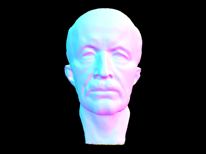
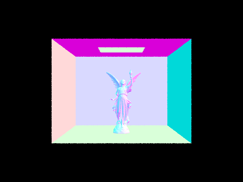
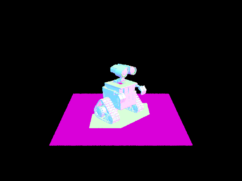
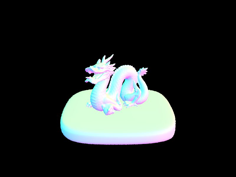
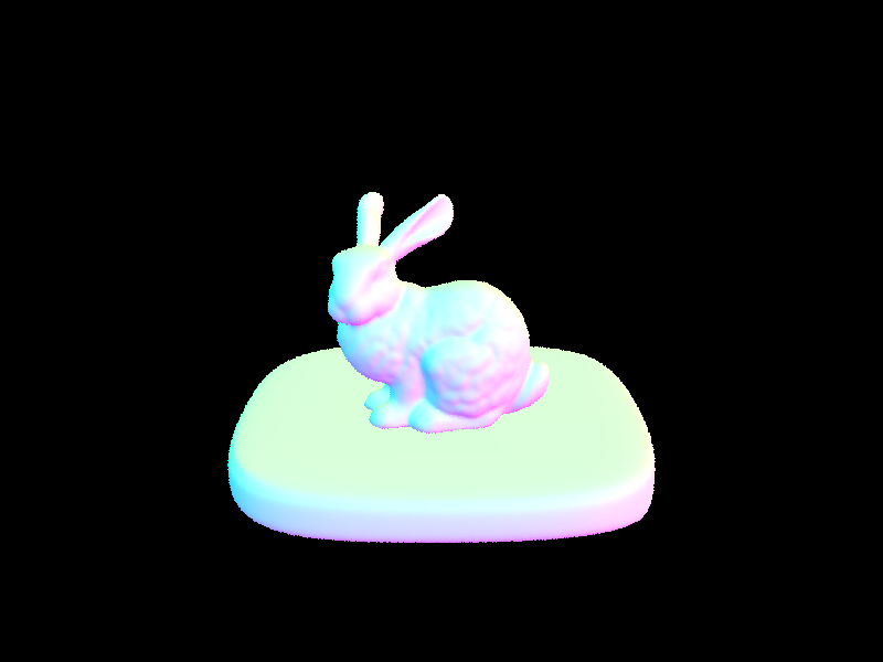
With BVH acceleration, our rendering times were much faster compared to before. For context, with BVH acceleration, rendering CBlucy.dae (133796 primitives) took just 0.0434 seconds, wall-e.dae (240326 primitives) took 0.0556 seconds, and dragon.dae (105120 primitives) took just 0.0478 seconds, while without BVH acceleration, CBlucy, wall-e, and the dragon were refusing to even render. The maxplanck.dae (50801 primitives) file took 277.7324 seconds to render without BVH acceleration (429788 rays traced and 8520.073848 intersection tests per ray averaged) but with BVH acceleration it took just 0.0600 seconds (341471 rays traced and averaged 2.728030 intersection tests per ray). Similarly, the bunny.dae (33696 primitives, 468895 rays traced, and 4526.5 intersection tests per ray averaged) took 136.66 seconds to render without BVH acceleration but with BVH acceleration, it only took 0.0660 seconds (363996 rays and 2.077795 intersection tests per ray averaged for the same number of primitives). Notice how for maxplanck.dae and bunny.dae, the number of rays traced and especially the number of intersection tests per ray reduced dramatically. This is because with BVH accelerations, we can reduce the number of rays we check on hitting primitives by using bounding boxes. We can just check if a ray hits primitives within a box, so we effectively use less ray intersection tests. We effectively reduced the ray intersection complexity from O(N) to just O(log(N)) which is a significant improvement.

Part 3: Direct Illumination (20 Points)

Walk through both implementations of the direct lighting function.

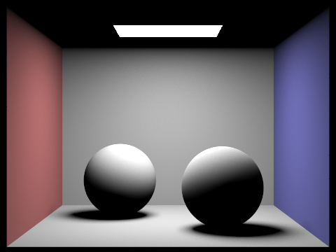
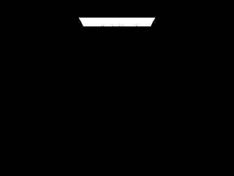
For direct lighting with uniform hemisphere sampling, we iterate over num_samples to calculate our Monte Carlo estimator. We then uniformly sample incoming ray directions in the hemisphere (let’s call this sample wj) using hemisphereSampler and get_sample(). We then calculate the PDF which is defined by 1.0 / (2.0 * pi). Next, we want to check if a new ray going from the hit_p in the sampled direction intersects a light source so we create a new ray (let’s call it newRay), which takes in hit_p for the origin and wj converted to world coordinates for the direction. We also set the newRay’s min_t to EPS_F to avoid numerical precision issues. We declare a new Intersection inter, which we pass in to bvh->intersect along with our newRay as our Ray and &inter as our Intersection. If there is a valid intersection, we can assume our new Intersection inter has been updated with the corresponding intersection point information. We pass w_out and wj converted back to object coordinates into isect.bsf->f() (this is our f_r in the Monte Carlo estimator), and multiply it by the emitted light from the new Intersection (L_i in the estimator) and multiplied by cos_theta of wj.unit() (cos_j in the estimator). Finally, we normalize (divide) by the PDF and add the resulting value to L_out. We repeat this process num_samples times and once we exit the for loop, we normalize L_out by num_samples before returning L_out.

For direct lighting by importance sampling lights, we first iterate through each SceneLight pointer in the scene->lights. We checked if the current light we are on is a point light source using is_delta_light(), and if true, then we can just sample once (all samples from a point light will be the same) and retrieve the emitted radiance by calling the current light’s sample_L(), and we pass in hit_p and the address of wi, distToLight, and pdf, the latter three of which we declared earlier in preparation for calling sample_L() since sample_L() writes into them (thus why we pass them in as addresses). We then want to create a new ray in order to perfect our ray intersection test with objects. We pass in hit_p as the origin and the rewritten wi by sample_L() as the direction to the ray. We then set the ray’s min_t and max_t while accounting for precision errors with EPS_F. We then want to check if there is no intersection between the newly created ray and objects in the scene using bvh->intersect(). If there isn’t an intersection and if cos_theta of wi.unit() (where all usages of wi from here on out has been converted to object coordinates since sample_L() rewrote it as world coordinates, let’s call this cos_j) is positive (Lambert’s Cosine Law), then we know that there was no other object between the hit point and the light source and we can assume the light source casts light on the hit point. As such, we can perform the same calculation as we did in task 3 (except we don’t normalize by number of samples). We take this resulting value and normalize by the PDF and add this to L_out. If the current light is not a point light source, then we should sample ns_area_light times (not all samples from the light will be the same, let’s call this num_samples). We do this by repeating exactly what we did above for when the light is a point light source, except now we repeat this num_samples times and after we exit the for loop, we normalize by num_samples. We repeat this for all the scene lights and afterwards we can return L_out.

Show some images rendered with both implementations of the direct lighting function.

Uniform Hemisphere Sampling	Light Sampling

Focus on one particular scene with at least one area light and compare the noise levels in soft shadows when rendering with 1, 4, 16, and 64 light rays (the -l flag) and with 1 sample per pixel (the -s flag) using light sampling, not uniform hemisphere sampling.

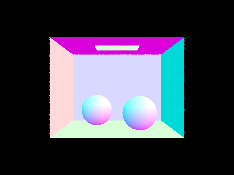
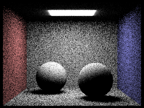
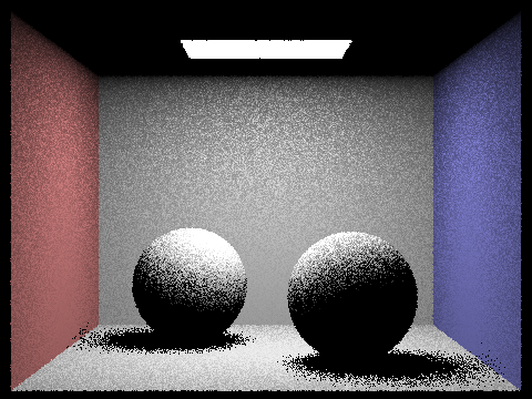
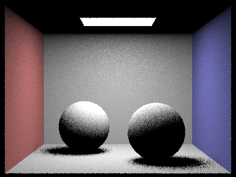
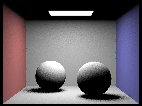
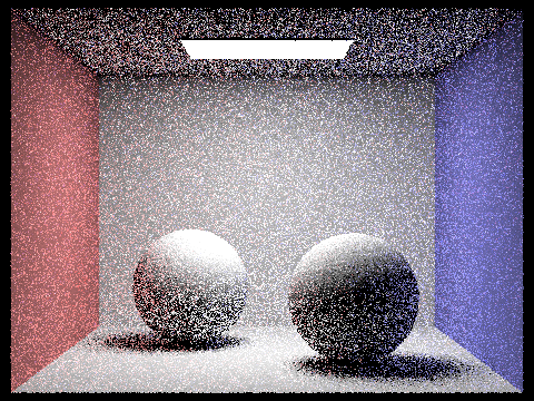
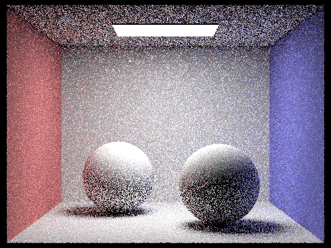
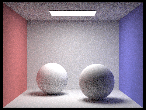
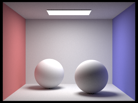
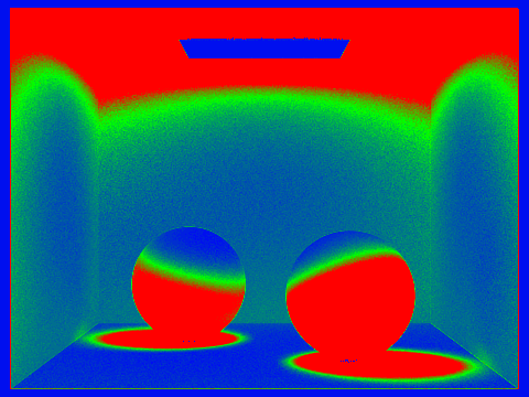
As we rendered with greater number of light rays, the soft shadows turned out smoother, more “condensed” (light rays 1 and 4 especially have noticeable soft shadows at the base of each sphere that extend to the wall and dont look “quite right”), and less noisy. This occurs because more light rays also means more samples from the light source have a better chance of hitting other areas besides intersecting with the objects.

Compare the results between uniform hemisphere sampling and lighting sampling in a one-paragraph analysis.

Uniform hemisphere sampling tends to be noisier than lighting sampling. This is because uniform hemisphere sampling takes uniformly random samples of rays, which means that some sampled ray intersects with an object while others don’t (only a certain chance of intersecting when random). This means for a lot of samples, we get a radiance of 0 which corresponds to grainy dark pixels and noisy looking images. Uniform hemisphere sampling also doesn’t do well with rendering scenes that have point light sources since the random uniform sampling method makes it so that there is a low chance of hitting the point light source (light source is small so low probability). For importance lighting sampling, we take samples from the light source itself which significantly reduces noise in images. When we sample directly from the light source itself, we reduce the number of rays that don’t contribute to the image as we can guarantee that the radiance of all our samples is greater than 0 (won’t get dark spots). In a way, when we do importance sampling lights, we are prioritizing the important rays, so we get smoother and much less noisy images for importance sampling.

Part 4: Global Illumination (20 Points)

Walk through your implementation of the indirect lighting function.

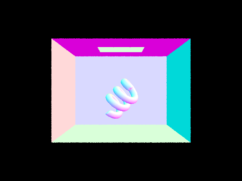
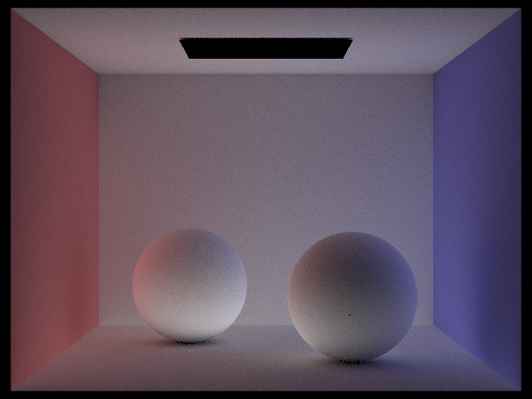
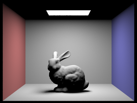
In order to render images with full global illumination, we build on our direct lighting function by adding support for indirect lighting. This way, we account for light reflected from other surfaces within the scene. We update est_radiance_global_illumination() so that it first calls zero_bounce_radiance(), then calls and adds the result of at_least_one_bounce_radiance(), which we implement as follows: First, we call one_bounce_radiance() to get the direct lighting at the given ray and intersection. Then, we check if the depth of this ray is less than or equal to 1. If so, then we terminate. Otherwise, we proceed. Using a static continuation probability (cpdf), we perform Russian Roulette, which terminates the function with probability 1 - cpdf. If the process doesn’t terminate, we compute the next bounce of the ray. We sample a BSDF value from the surface intersection point using isect->bdsf.sample_f(), and generate a new ray and intersection point, with the new ray depth being one less than the current ray. We check if the new ray intersects the bvh. If the ray intersects, we recursively call at_least_one_bounce_radiance() on the new ray and apply the reflectance formula onto the result, which gets added to the total indirect illumination. Finally, the function returns the total indirect illumination.

Show some images rendered with global (direct and indirect) illumination. Use 1024 samples per pixel.

Pick one scene and compare rendered views first with only direct illumination, then only indirect illumination. Use 1024 samples per pixel. (You will have to edit PathTracer::at_least_one_bounce_radiance(...) in your code to generate these views.)

For CBbunny.dae, compare rendered views with max_ray_depth set to 0, 1, 2, 3, and 100 (the -m flag). Use 1024 samples per pixel.

Pick one scene and compare rendered views with various sample-per-pixel rates, including at least 1, 2, 4, 8, 16, 64, and 1024. Use 4 light rays.

Part 5: Adaptive Sampling (20 Points)

Explain adaptive sampling. Walk through your implementation of the adaptive sampling.

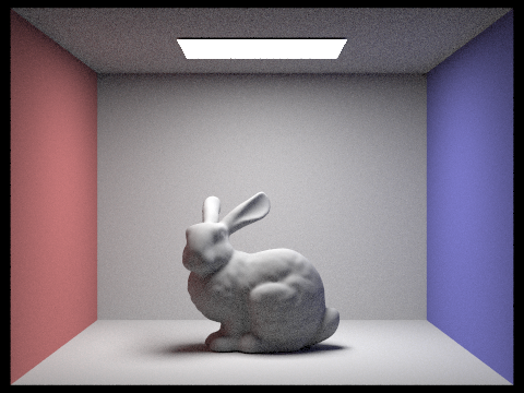
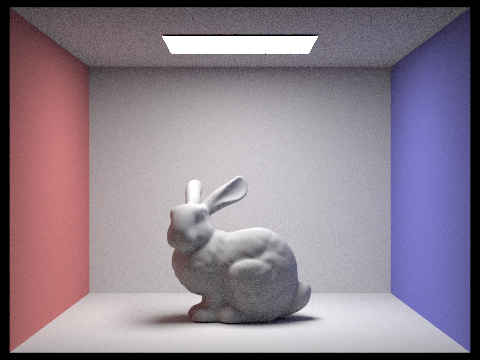
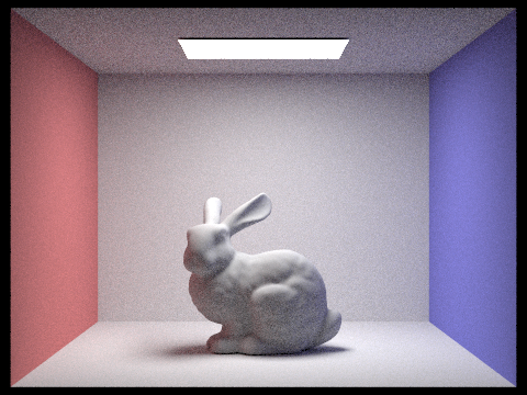
As seen in the previous parts, Monte Carlo path tracing is useful in generating realistic images, but it can result in a lot of noise. ​​Increasing the number of samples per pixel can reduce the noise, but this isn’t the best solution. Adaptive sampling is an optimization technique that modifies the sample rate of a pixel based on how quickly the pixel converges. This allows us to avoid uniformly sampling all pixels at the same high rate. Instead, we perform less sampling on pixels that converge faster and more sampling on pixels on more difficult areas of the image. To implement adaptive sampling, we updated our raytrace_pixel() method to include a simple algorithm. We define two variables, s1 and s2 and initialize them to 0. Then, when looping through the total number of samples, we take the illuminance of each sample, then accumulate the illuminance and illuminance squared to s1 and s2, respectively. Using s1 and s2, we calculate the mean and standard deviation each time we reach a certain sample threshold, i.e. every time samplesPerBatch iterations. Then, we divide the standard deviation by the number of samples so far to calculate the pixel's convergence. If the pixel’s convergence is less than or equal to maxTolerance times the mean, then the pixel converges, and we terminate the loop early. Otherwise, we continue as usual.

Pick two scenes and render them with at least 2048 samples per pixel. Show a good sampling rate image with clearly visible differences in sampling rate over various regions and pixels. Include both your sample rate image, which shows your how your adaptive sampling changes depending on which part of the image you are rendering, and your noise-free rendered result. Use 1 sample per light and at least 5 for max ray depth.

Reflection

Project 3-1 was definitely challenging, in terms of the content and implementation, as well as being able to balance this task with our other projects and midterms; but we did our best to work together collaboratively all the way through. We worked together largely for parts 1 and 2 by meeting in-person during project parties or online synchronously through Discord. For parts 3 through 5, we saw a lot more conflicts within our schedules, so we primarily worked asynchronously, updated each other on our progress, and made sure to push our code with comments to the shared repository so that the other person would reference and ask questions. Towards the end, when we had more matching availability again, we were able to communicate more and work through bugs together, since a lot of the bugs we faced in the later parts of the project stemmed back from our implementation in earlier parts. We found out that there was a “Code with Me” feature in CLion after we completed our project code, which would have been helpful for this project as well as earlier ones, but moving forward with future projects, we definitely see this as a viable tool that will help us collaborate more efficiently. Throughout this project, we learned a lot about ray tracing and illumination, as well as different optimization methods.