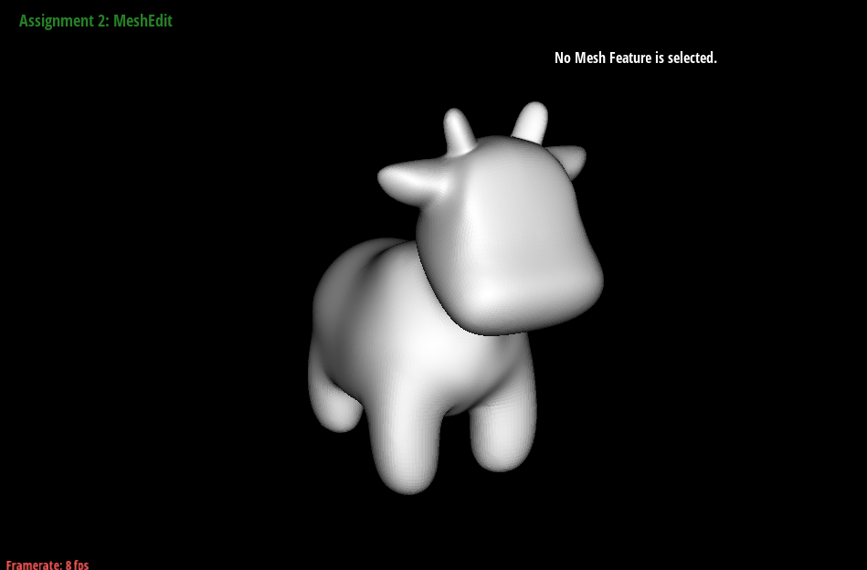
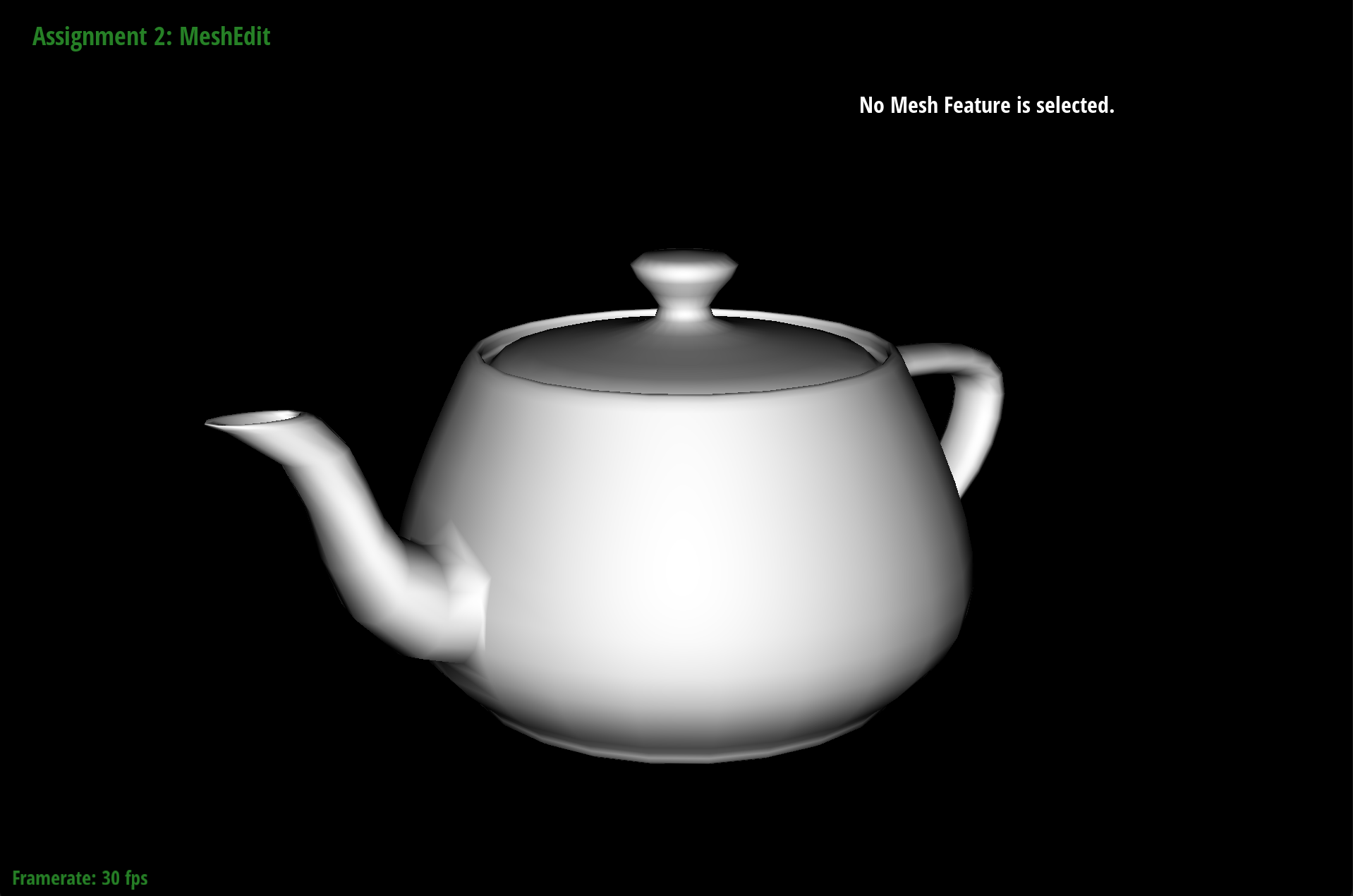
In this assignment, we implemented a mesh editor that can handle a variety of mesh operations. We first started by building Bezier curves using de Casteljau’s algorithm then we extended the use of the algorithm to Bezier surfaces. We then worked with manipulating triangle meshes through the half-edge data structure, and implemented area-weighted vertex normals which would allow for smoother shading and implemented operations such as edge flipping and edge splitting. Edge flipping and edge splitting would come in handy for our implementation of loop subdivision, which is a mesh upsampling method which would allow for higher-resolution meshes. At the end, we now have a working mesh editor that is capable of area-weight vertex normals, flipping edges, splitting edges, and upsampling the current mesh.
We learned from this assignment how meshes are handled in 3D modeling and animation software programs such as Maya and Blender, and what truly goes on behind the scenes when we choose the number of subdivisions for our meshes, what happens when we delete/add an edge, and the underlying data structures that might have been used for those software programs.
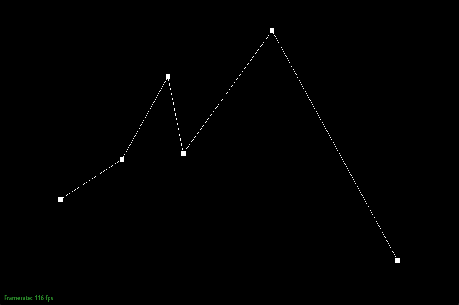
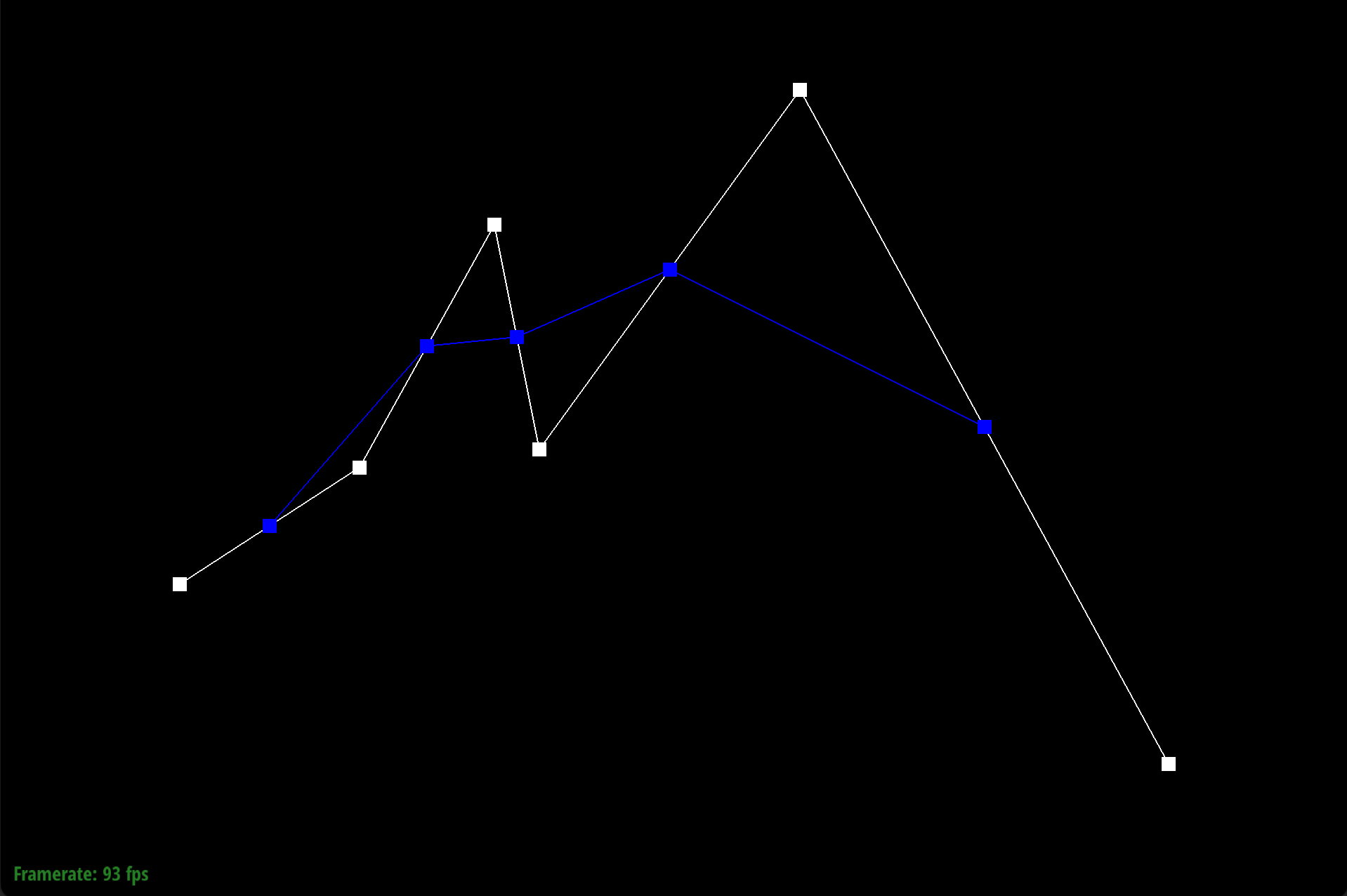
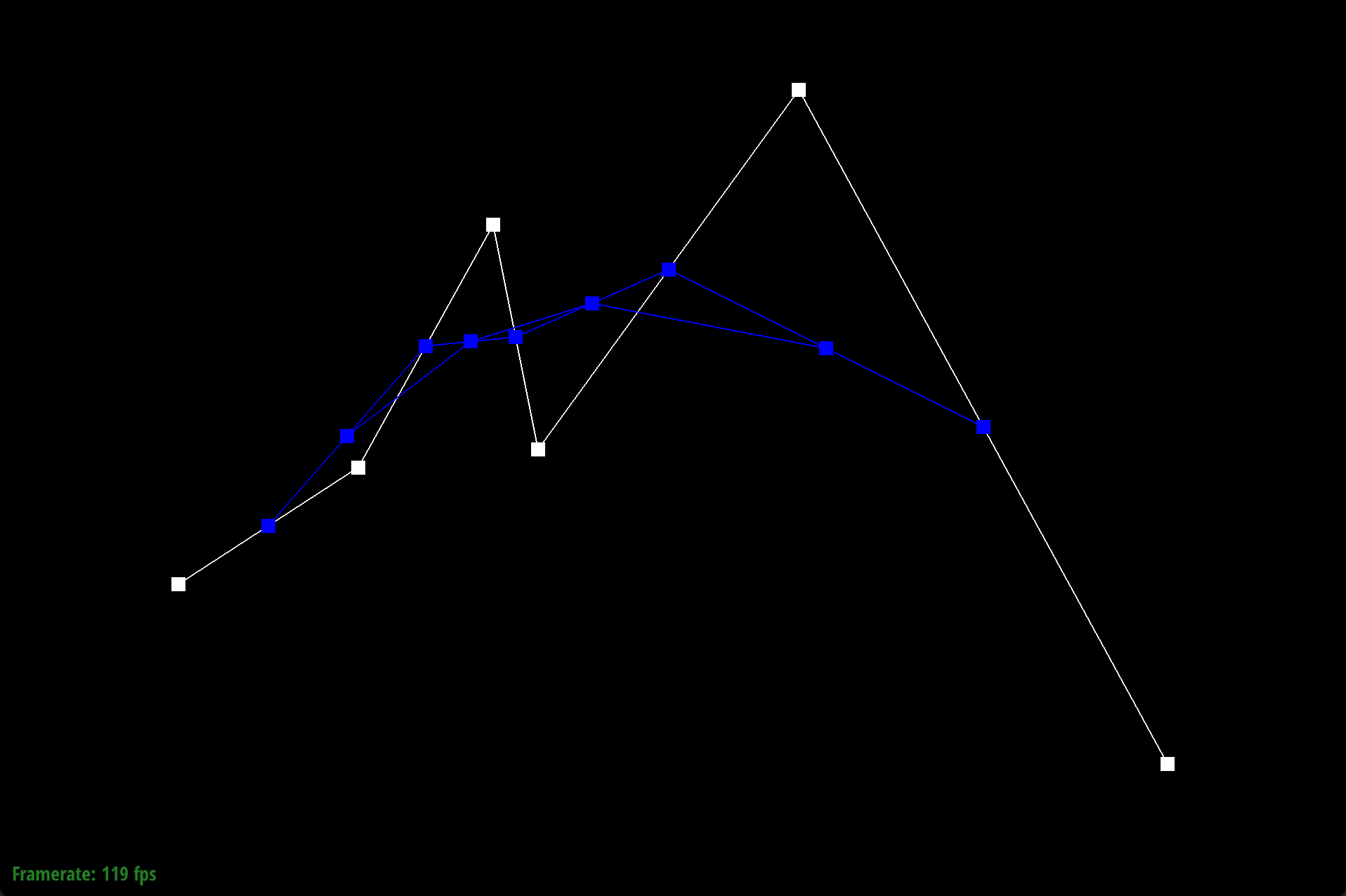
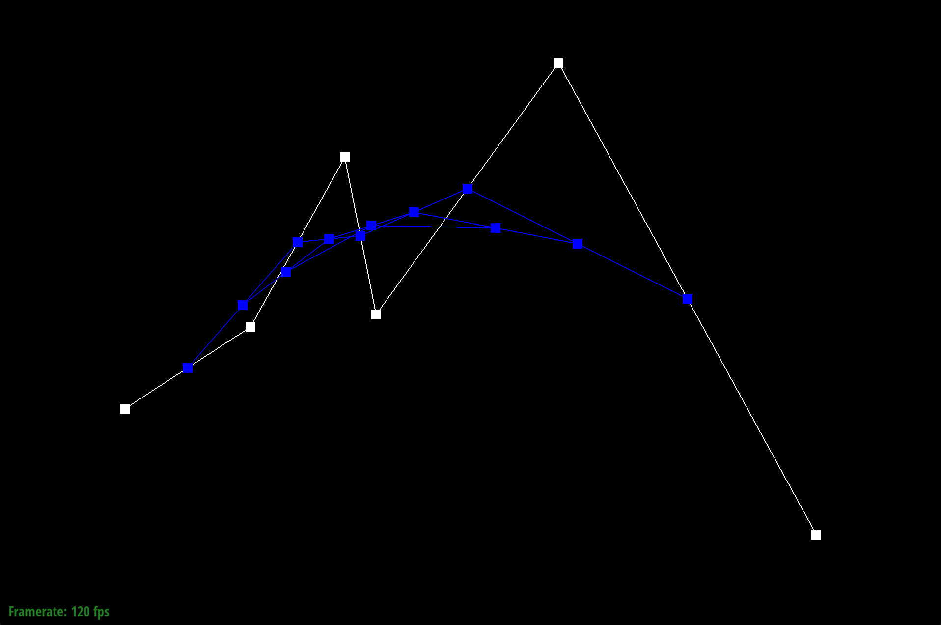
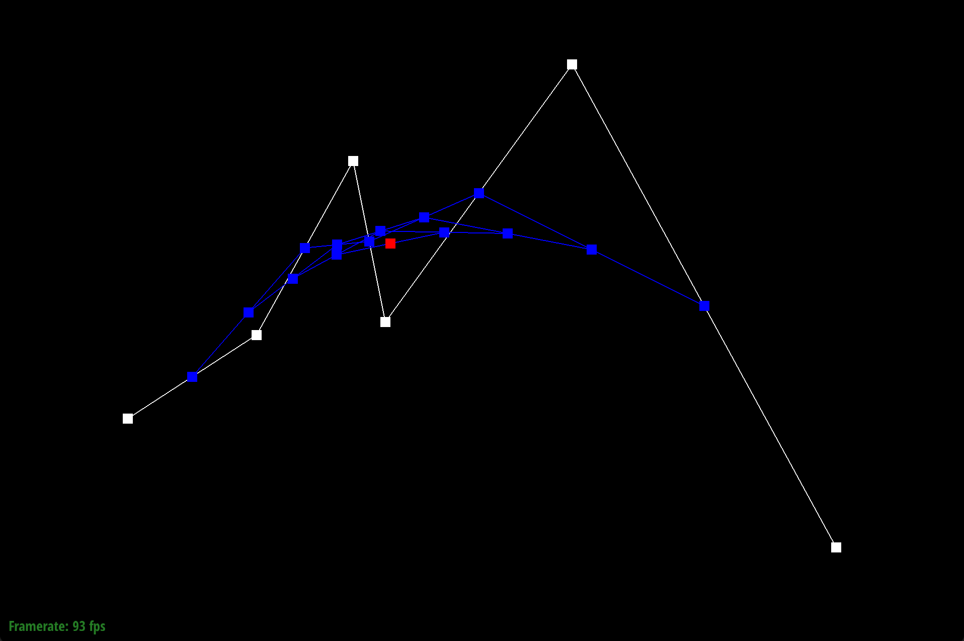
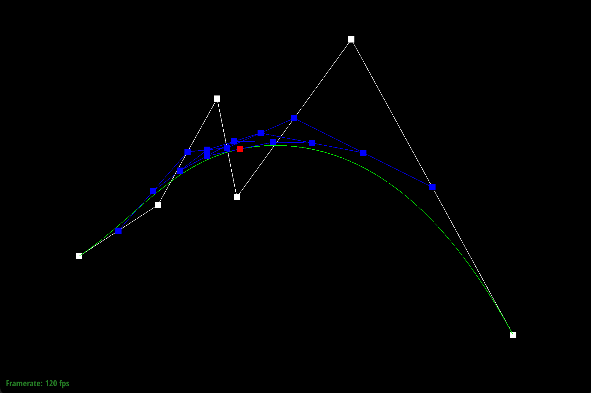
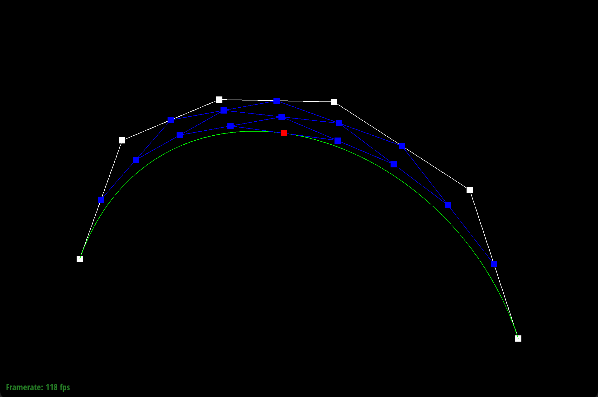
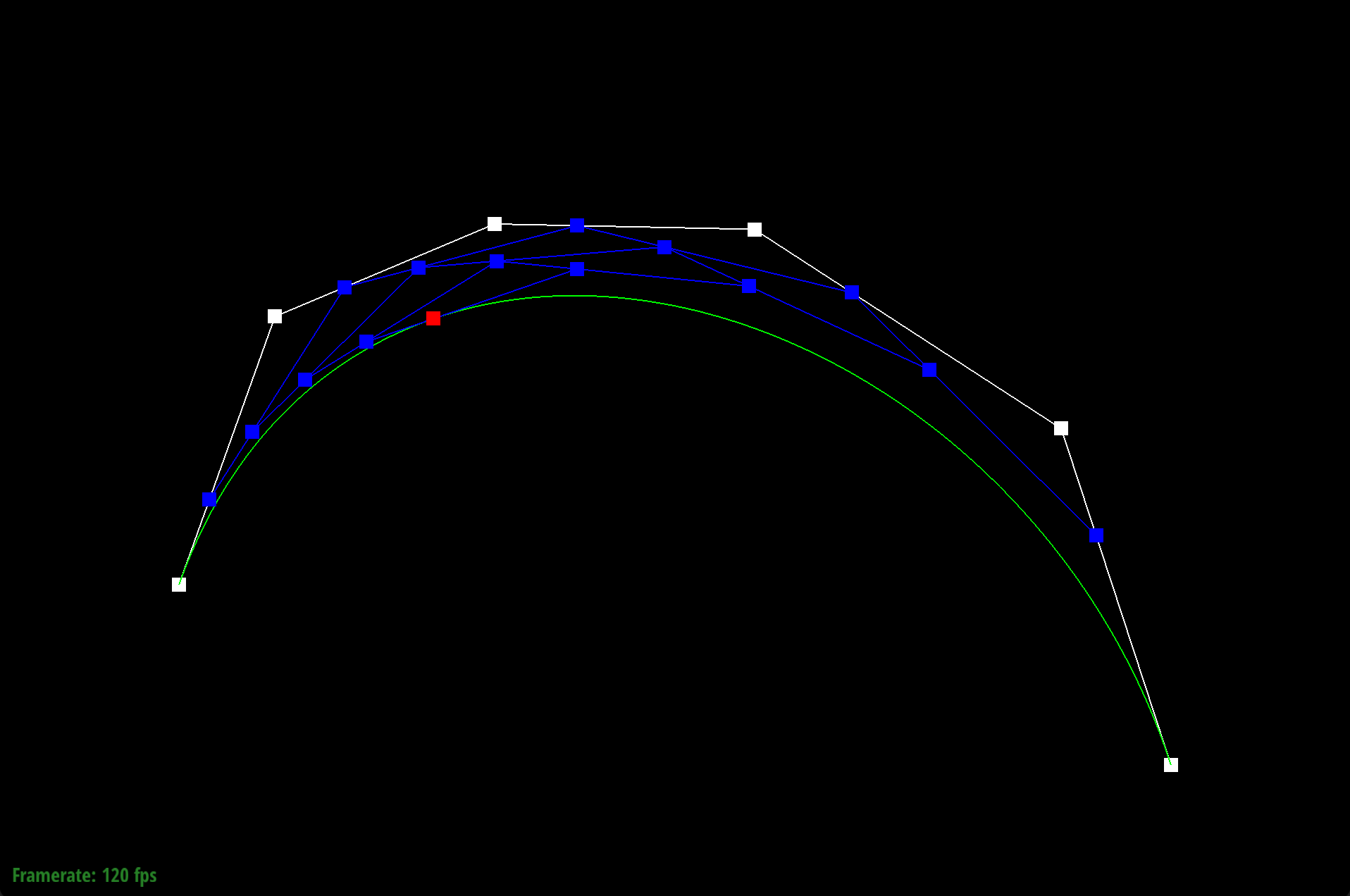
De Casteljau’s algorithm works through a series of recursive steps. Using n control points and a parameter $t$, we use linear interpolation to compute $n-1$ intermediate control points at parameter t in the next subdivision level. Visually for bezier curves, we use linear interpolation to insert a point and an edge. If we recursively repeat this process, we will converge to a final single point that lies on the Bezier curve at parameter $t$, which defines our final curve. For our implementation of de Casteljau's algorithm, we began by creating an empty standard vector of Vector2D objects that would store the $n-1$ intermediate control points at parameter $t$ in the next subdivision level. Using a for loop, we iterated through the given n control points from $p_1$ to $p_{(n-1)}$ and performed linear interpolation, computing $p'_i = (1-t)p_i + tp_i$, where $p'_i$ is an immediate control point at parameter t of the next subdivision level. We do not include $p_n$, as no $p_{(n+1)}$ exists for the linear interpolation computation. With each computation, we appended $pi’$ to our vector of immediate control points. Once the for loop finishes, we return our vector of $n-1$ intermediate control points.
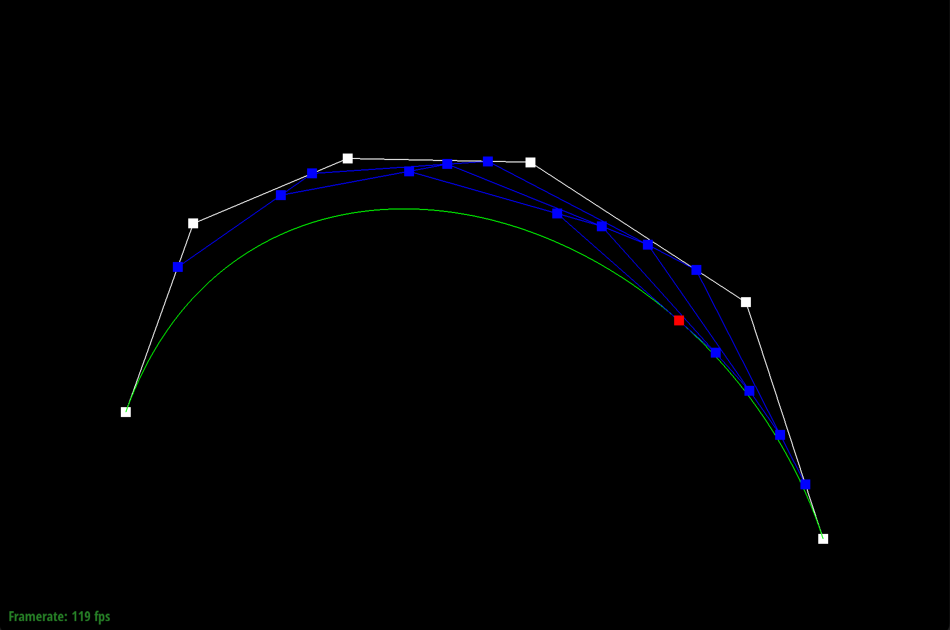
We defined our Bezier curve at control points (0.200, 0.350), (0.400, 0.480), (0.550, 0.750), (0.600, 0.500), (0.890, 0.900), and (1.300, 0.150).
|
|
|
|
|

|
|
|
|
Similar to Bezier curves, de Casteljau’s algorithm extends to Bezier surfaces by working with an n x n grid of control point vectors through a series of recursive steps. Instead of just working with one parameter t, this time we work with parameters u and v. The intuition is that each row in the n x n grid gives us a set of control points that defines a Bezier curve at parameter u. Applying de Casteljau’s algorithm to each row in the grid gives us a total of n Bezier curves, and likewise, a vector of n evaluated points, which creates a “moving curve” in 2D space. We can then use 1D de Casteljau to evaluate the Bezier curve provided by this “moving curve” at parameter v and return a point on the Bezier surface in 3D space.
To apply de Casteljau algorithm to Bezier surfaces, we implemented three functions: evaluateStep(...), evaluate1D(...), and evaluate(...).
We used the same logic from Task 1 in our implementation of evaluateStep(...), but since we are working with points in 3D spaces, we stored our intermediate control points in a vector of Vector3D objects. Within evaluate1D(...), we continuously called evaluateStep using a while loop, which terminated once the evaluateStep returned a vector of size 1. Then, we retrieved the Vector3D element, by returning the element at index 0 in the vector returned by evaluateStep.
On the highest level, our evaluate(...) method implementation begins with initializing a standard vector of Vector3D objects to contain the moving curve points, i.e. the set of single points evaluated at each Bezier curve given by each row within our nxn grid of control points. Then, we iterated through the rows of control points using a for loop from 0 to n. With each iteration, we called evaluate1D with inputs being the vector of control points given by row i and parameter u. This gave us the single final, single point P_i for the i-th row, which we stored in the vector of moving curve points created earlier. Lastly, we evaluated evaluate1D with the vector of moving curve points and parameter v as inputs, which returned the surface point.
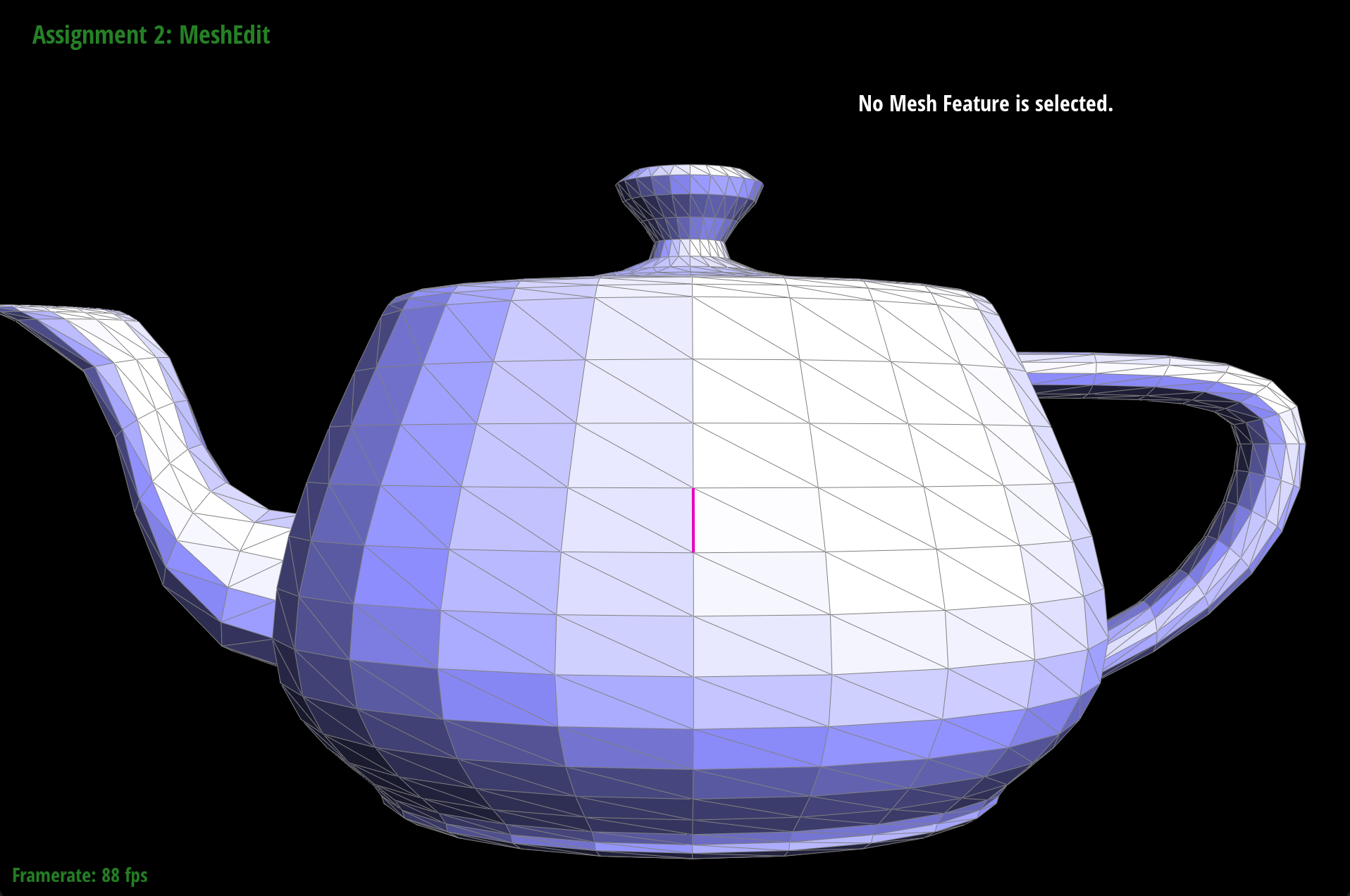
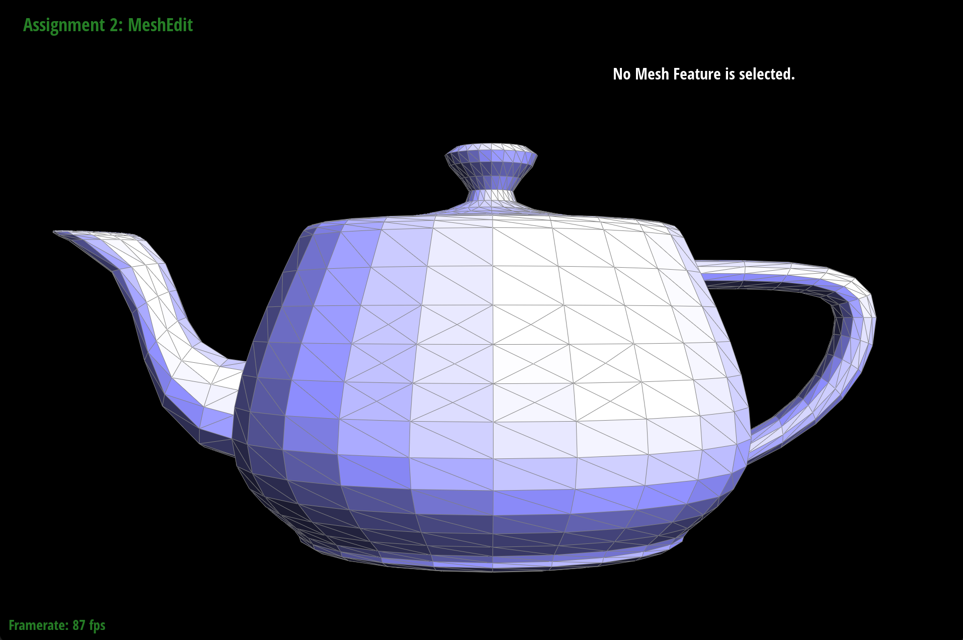
To implement the area-weighted vertex normals, we began by initializing a Vector3D of zeros, which we use to sum the weighted normals of each face incident to the vertex. Then, we got the reference halfedge to this vertex by calling halfedge(). Using a do-while loop, we iterated through each halfedge incident to the vertex under the condition that the current halfedge is not our reference halfedge. While the condition is true, we first check if the face of the halfedge is in the boundary. We add the weighted normal of the face only if the face is not in the boundary.
To get the weighted normal of each face, we compute the area of the face then multiply it by the normal of the face. Area is computed by taking the cross product of two edges and dividing by 2. So, we retrieve the position of the three vertices of the triangle. The first vertex, v1 is the given vertex, which we get the position for using the Vector class member variable position. To get the second vertex, v2, we retrieve the next halfedge to the current one, retrieve the vertex of this next halfedge, then take the class member variable position for that vertex. To get the final vertex, v3 we do the same thing, but take the next halfedge of the next halfedge.
Once we had all three vertex positions, we took the cross product of two edge vectors, given by v2 - v1 and v3 - v1, then take the Euclidean norm if the resultant vector. Then, we divide by 2 to get the area of the face. We use this area to weigh the normal of the face for the current halfedge by multiplying the two values. After, we add the result to our Vector3D variable outside of the loop, that is keeping track of the current sum of weighted normals.
To proceed to the next iteration, we reassign the current halfedge to be the next halfedge of the twin of this halfedge. Once we end up back at the original reference halfedge, the do-while loop terminates. At this point, we’ve summed all weighted normals of the faces incident to the given vertex.
Our last step is to return the normalized sum of all area-weighted normals, which we do by calling .normalize() on our weighted normal sum variable. Then, we return the variable.
|

|
|
|

|
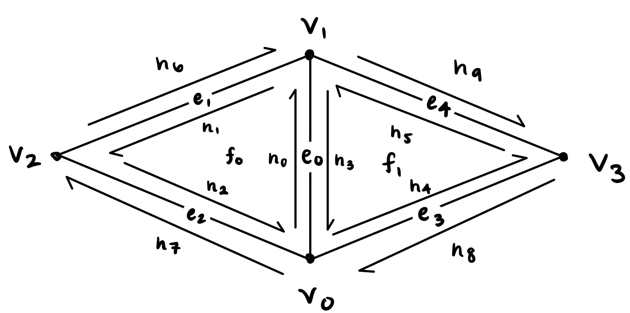
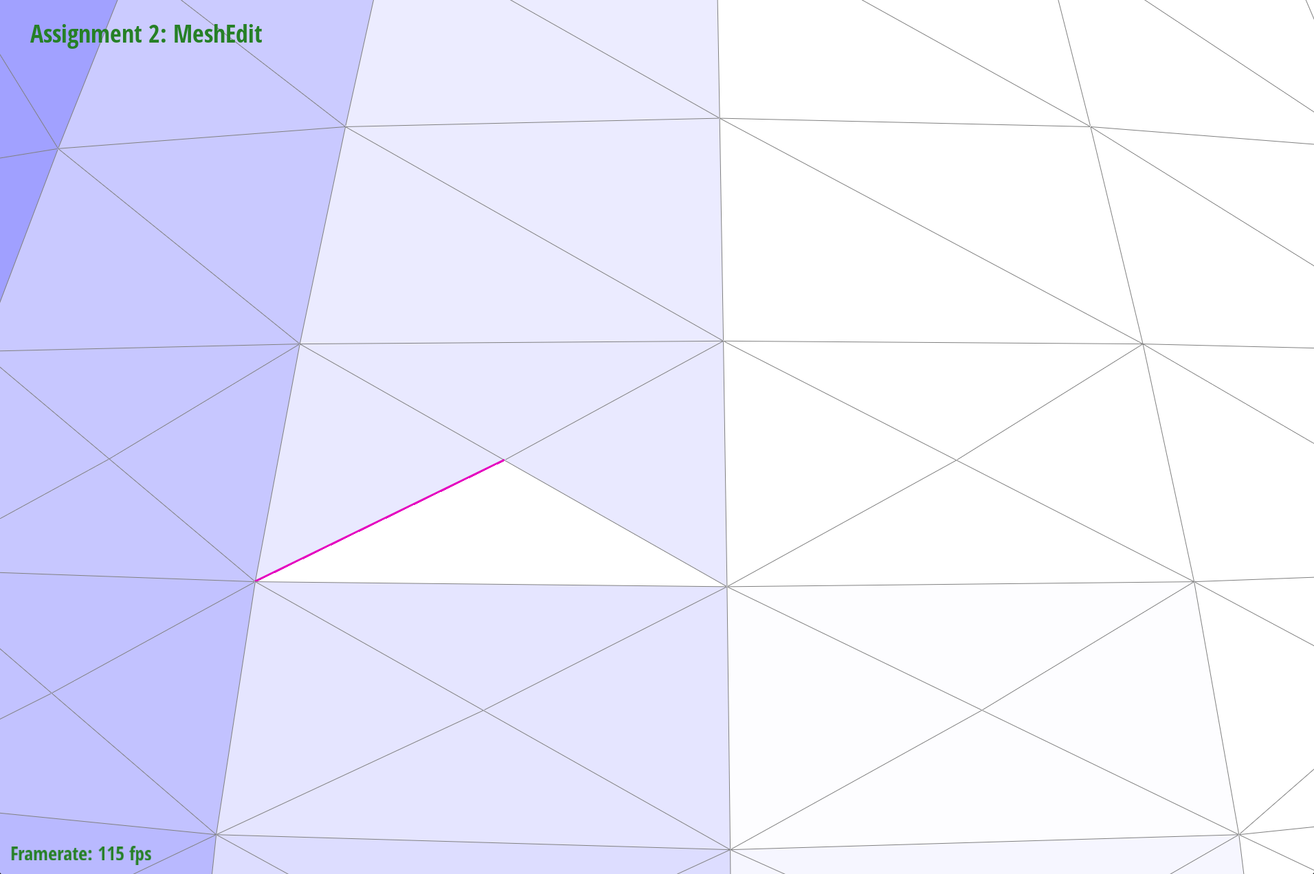
The edge flip operation should flip the given edge and return an iterator to the flipped edge. For our edge flip implementation, we know that the function should return immediately if either neighboring face of the edge is on a boundary loop. So, we begin with a simple condition statement checking the neighboring faces. If the inputted EdgeIter is on the boundary, then we return the same EdgeIter. Otherwise, we perform the edge flip operation.
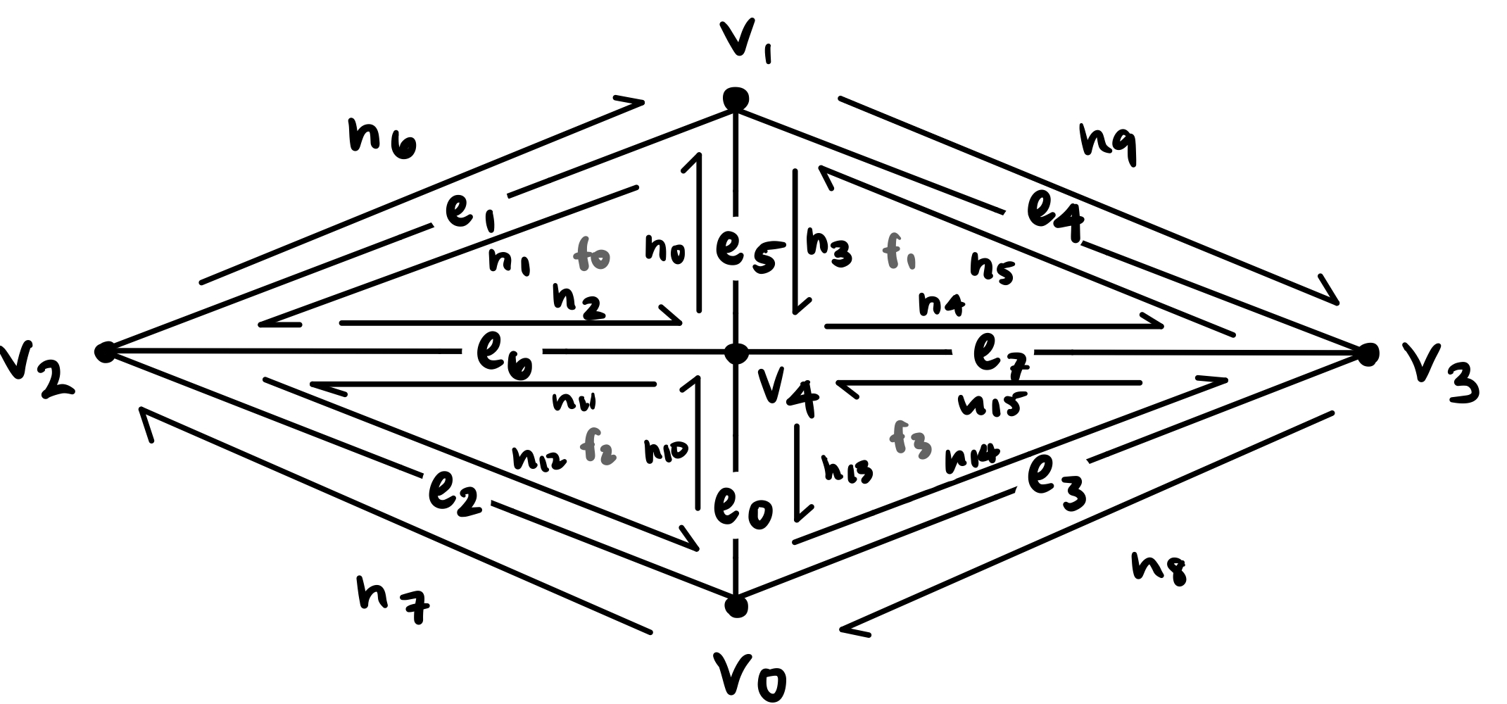
To perform the edge flip, we first drew out what our triangle mesh looks like, as depicted below. Then, we assigned all the mesh elements to variables that matched our image, so that we can easily identify each mesh element for reassignment after the edge flip. We created a HalfedgeIter for each of our halfedges h0, h1, ..., h9; a vertexIter for each of our vertices v0, ..., v3; a EdgeIter for our edges e1, ..., e4. For faces, we assigned f0 and f1 to corresponding faces based on the corresponding halfedges (h0 and h3 were pointers to faces f0 and f1 respectively). At this stage, we have not performed edge flipping yet.
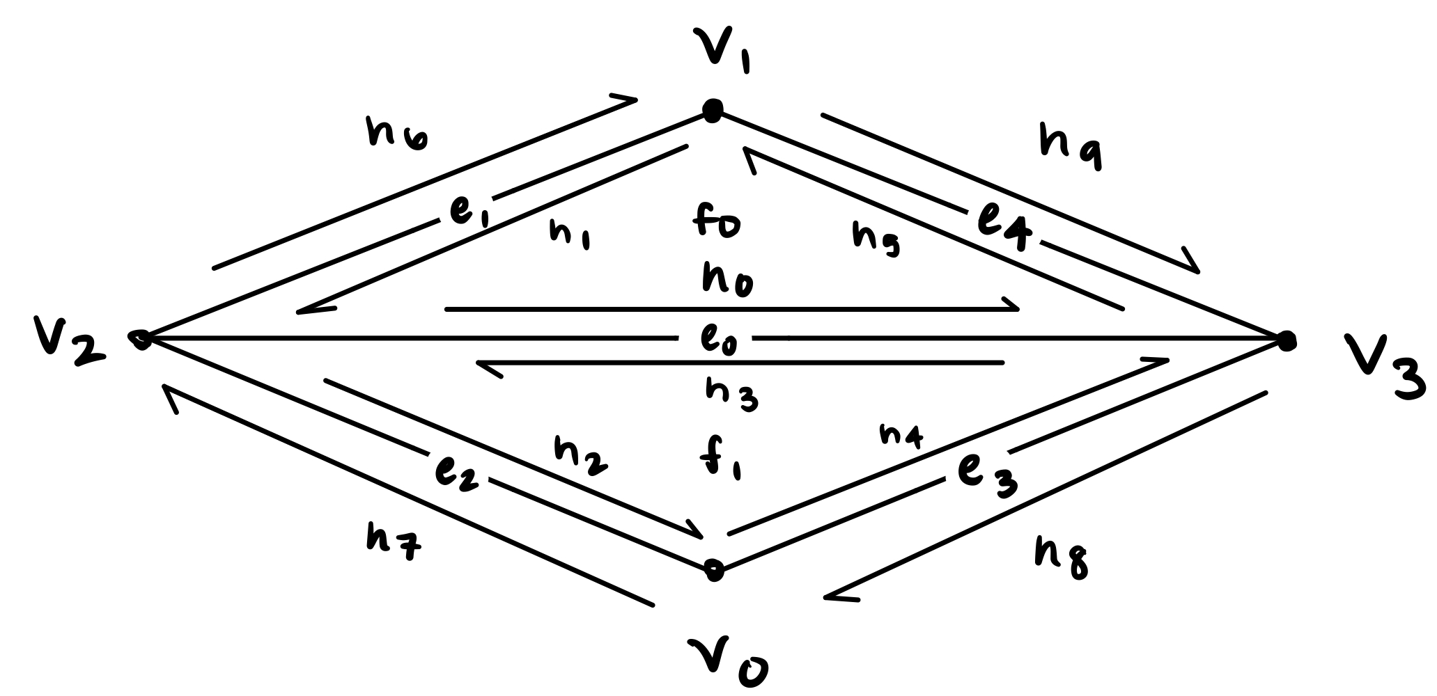
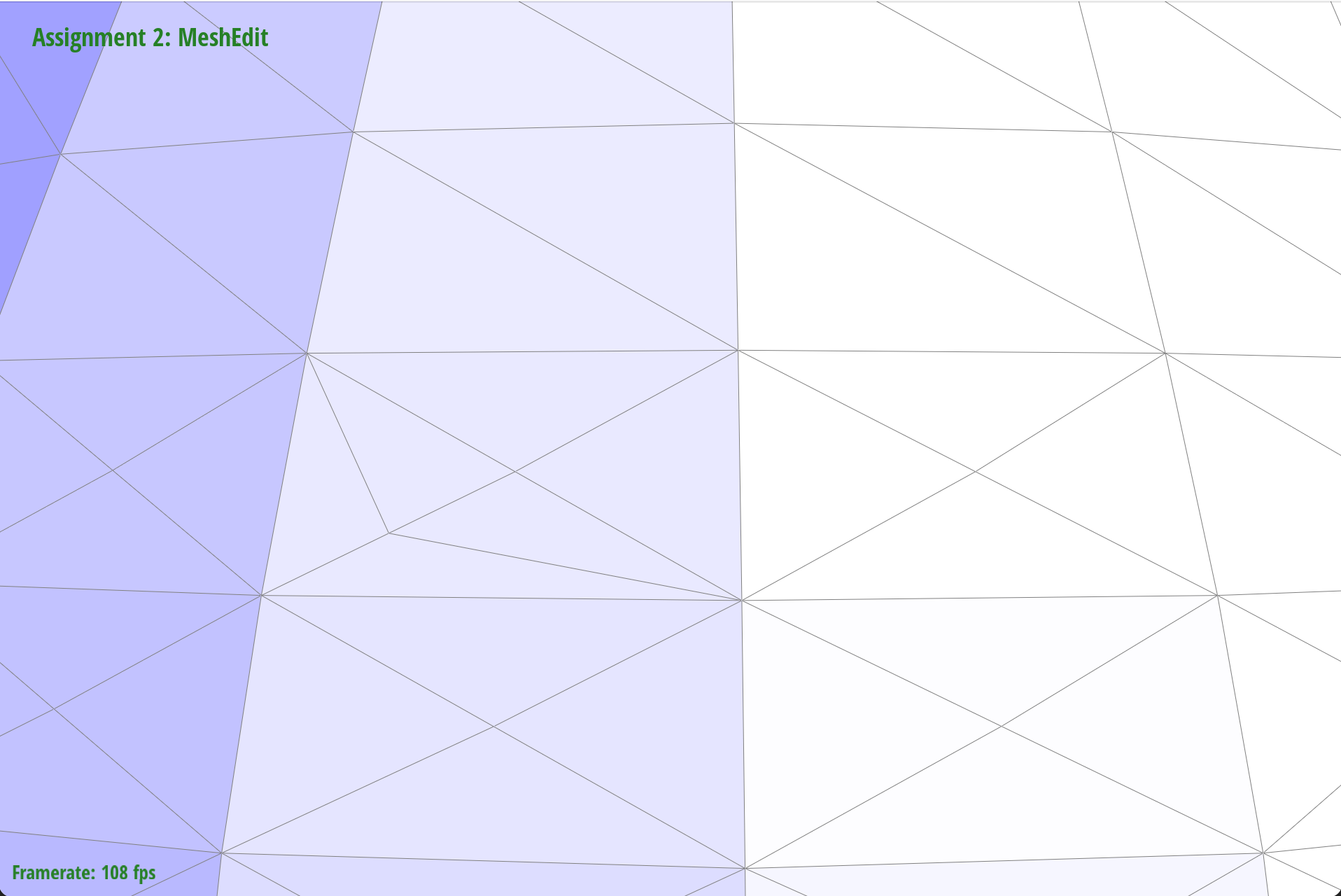
For the actual edge flipping, we then drew our what the triangle mesh looks like after flipping, also depicted below. Based on this new image, we reassigned pointers for each halfedge, vertex, edge, and face struct. For every halfedge h0, h1, …, h9, we used setNeighbors() to set all the new pointers to the new next halfedge, the new twin halfedge pointer, the new vertex pointer, the new edge pointer, and the new face pointer. For every vertex, edge, and face, we set the new corresponding halfedge pointer.
|
|
|
|
|
|
When we flipped diagonal edges, the edges would disappear; it didn’t appear to be working correctly. However, when we flipped vertical or horizontal edges, the flips appeared to work correctly. To debug this, we drew out various diagrams and checked our pointers. When we flipped edges in the GUI, we checked to see if the outcome matched what we expected. Since only diagonal flips weren’t working, we suspected something was wrong with the corresponding “outer” halfedges or edges. Turns out this assumption was correct, and there was a small bug with assigning the halfedges and edges correctly due to a mix up in the diagram and redrawing the diagram helped to catch this error.
The edge split operation should split the given edge and return an iterator to the newly inserted vertex. Similar to our edge flip operation, we began with a conditional statement. If the inputted EdgeIter is on the boundary, then we return the VertexIter given by the halfedge of this inputted edge by default. Otherwise, we perform the edge split operation.
Again, we first drew out what our triangle mesh looks like. Then, we assigned all the mesh elements to variables that matched our image, so that we can easily identify each mesh element for reassignment after the edge split.
We then drew out what our triangle mesh would look like after the operation. Splitting a given edge involves the addition of new mesh elements, so we create new mesh elements as needed. Specifically, our edge split implementation called for the addition of 6 halfedges, 1 vertex, 3 edges, and 2 faces. Additionally, the vertex element we created is the newly inserted vertex that needs to be returned. We had to assign the position of the new vertex to the midpoint of the original edge. To get the midpoint, we added the position vectors of v0 and v1, then divided the sum by 2. We assigned this result as the position of the new vertex. Afterward, we reassigned all pointers of mesh elements, regardless of whether they were updated or not, as according to our drawing.
|
|
|
|

|
|
|
|
|
|
|
|
|
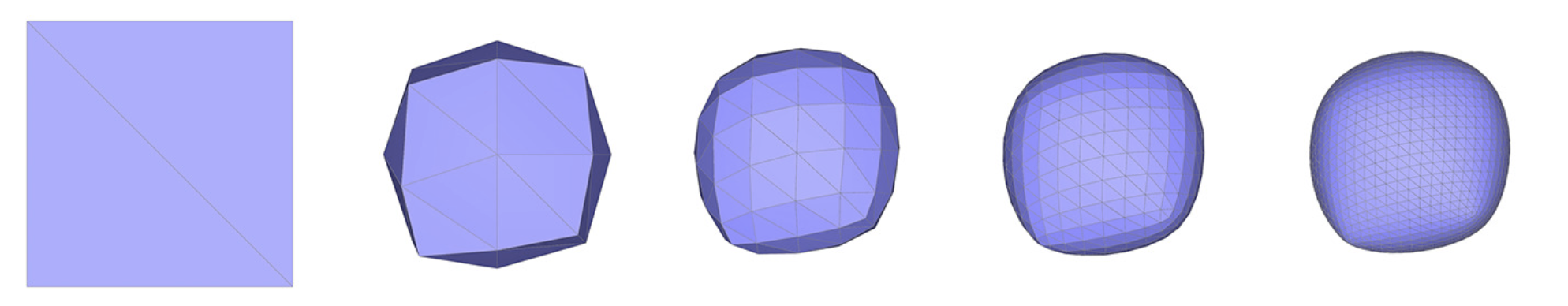
Our loop subdivision consisted of three parts:
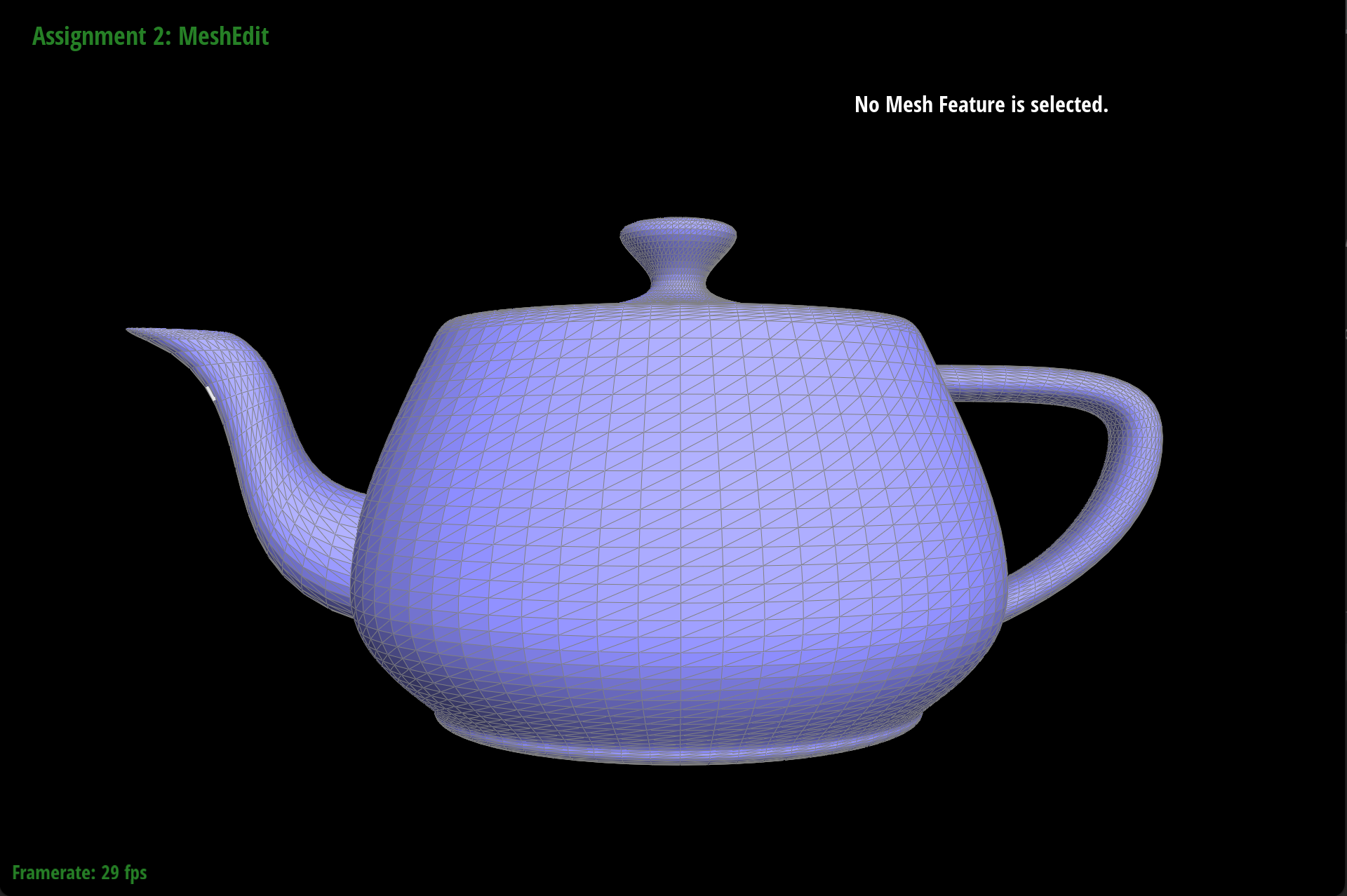
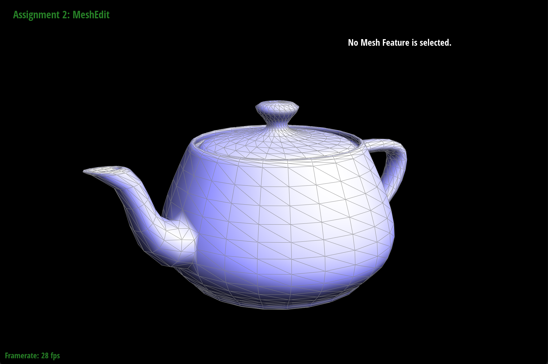
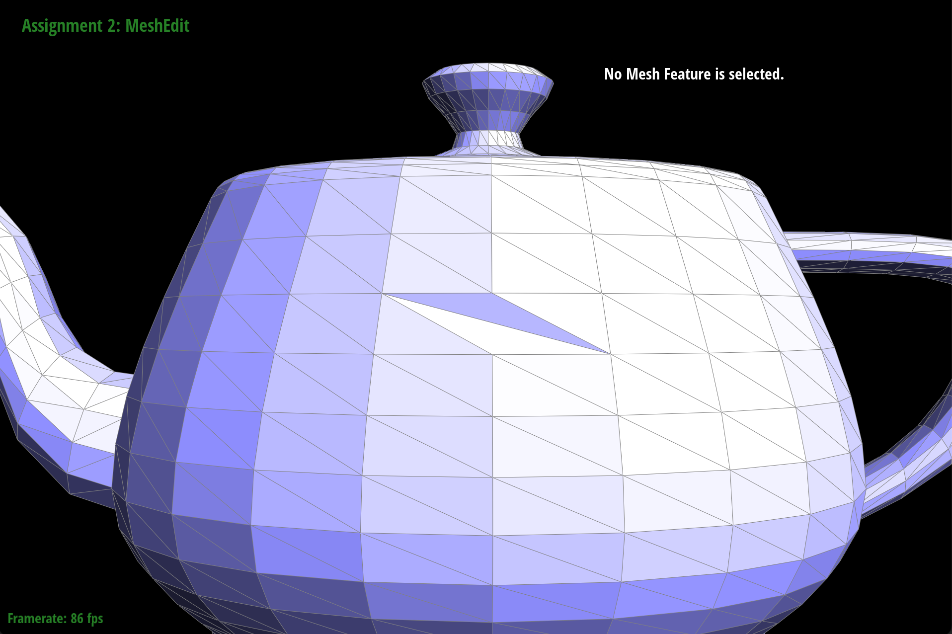
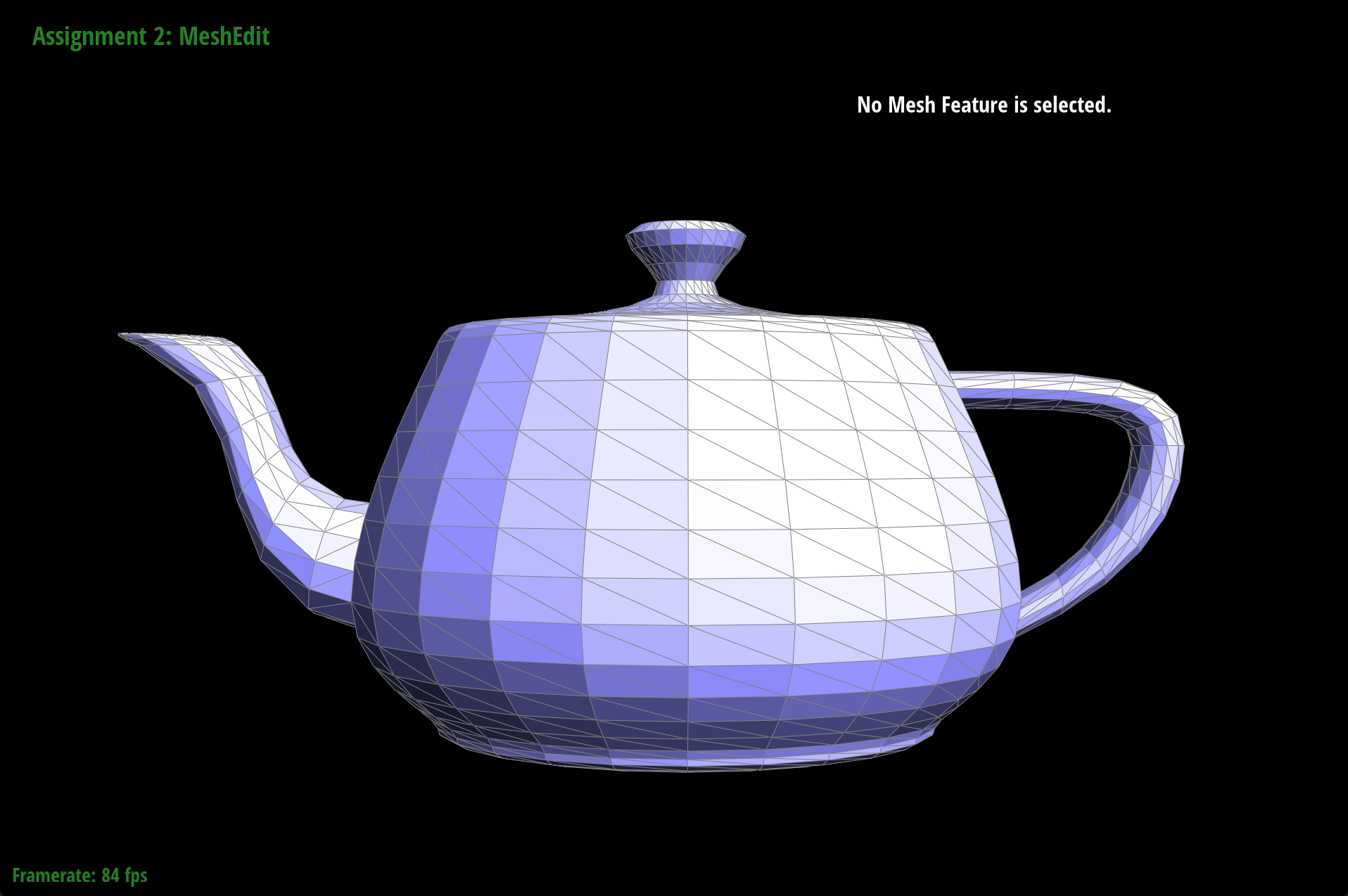
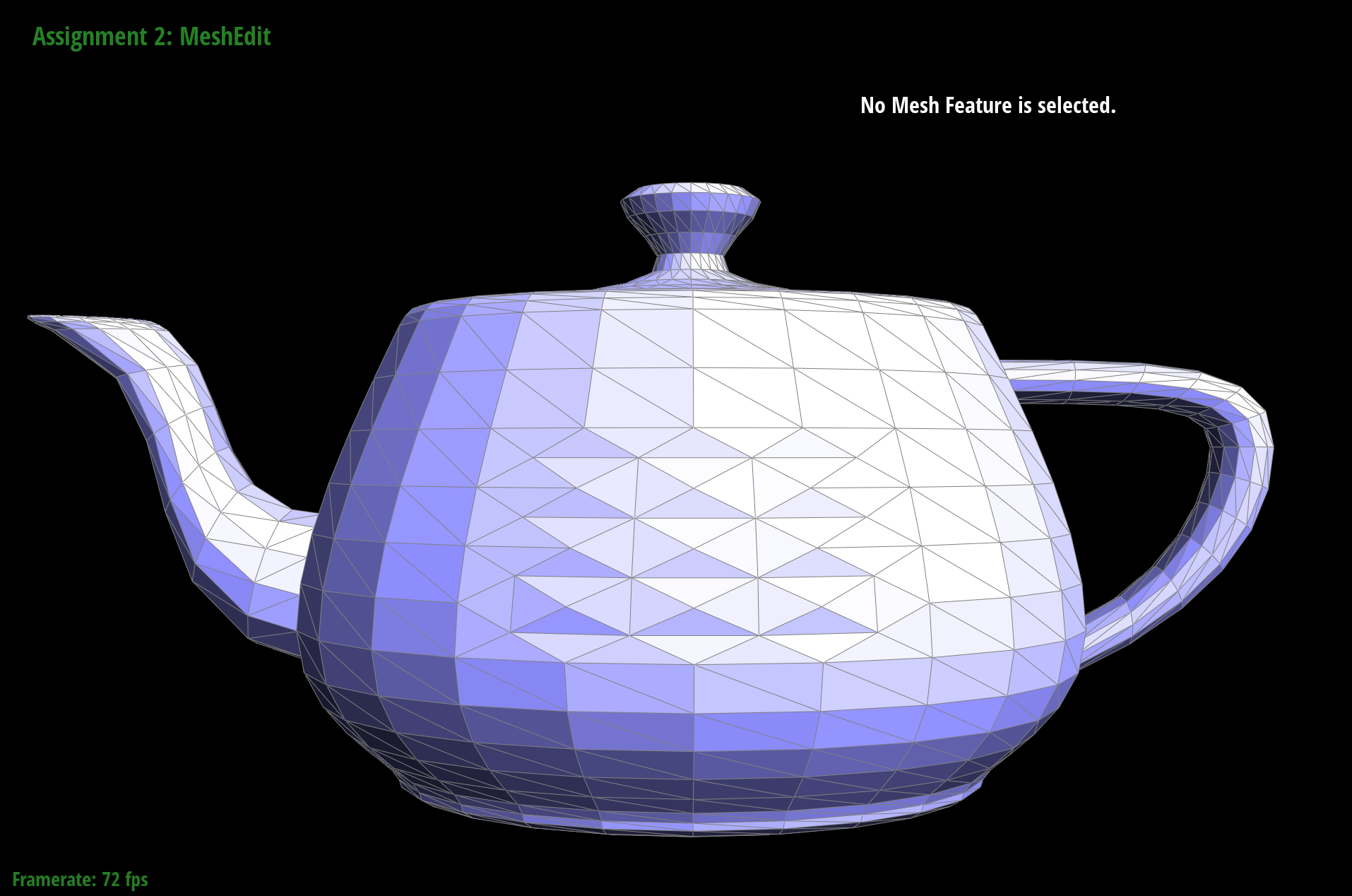
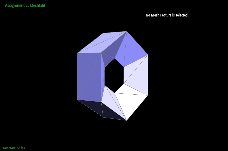
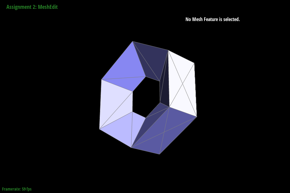
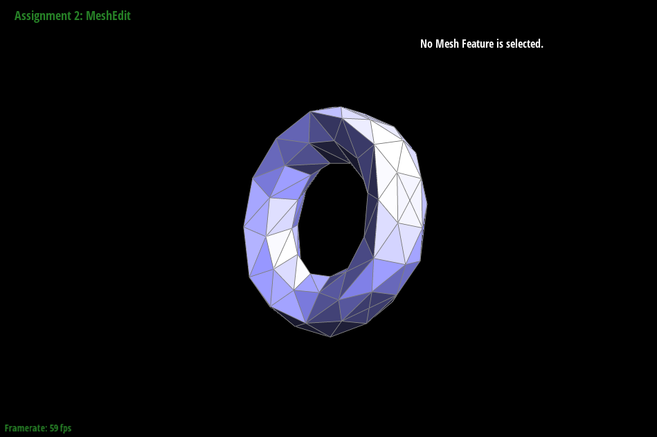
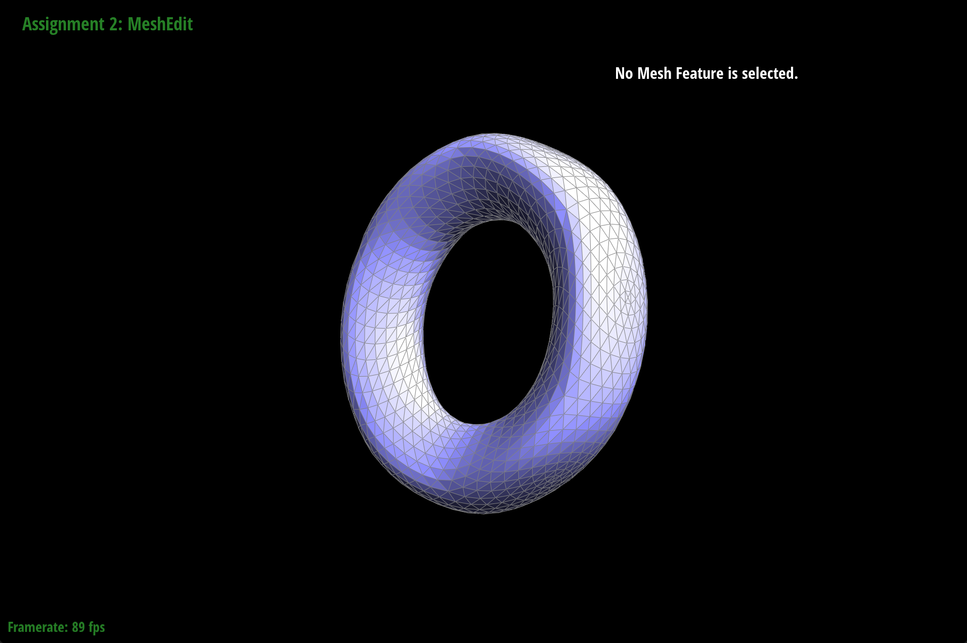
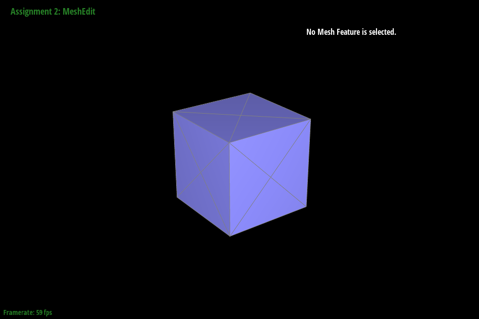
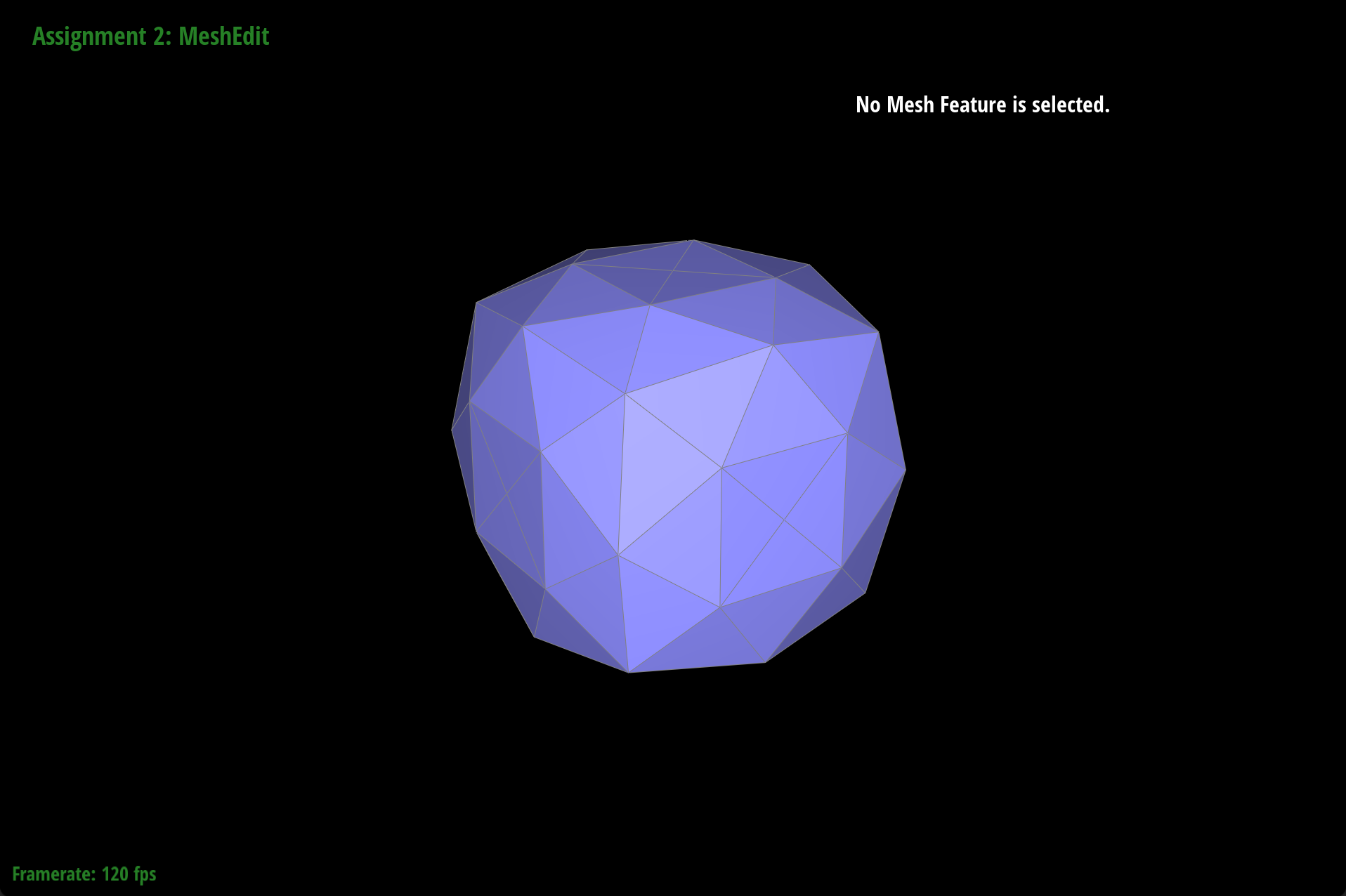
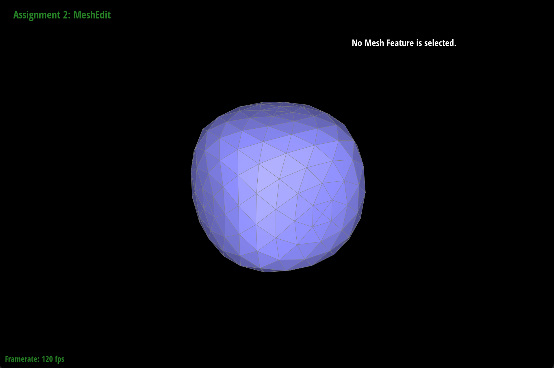
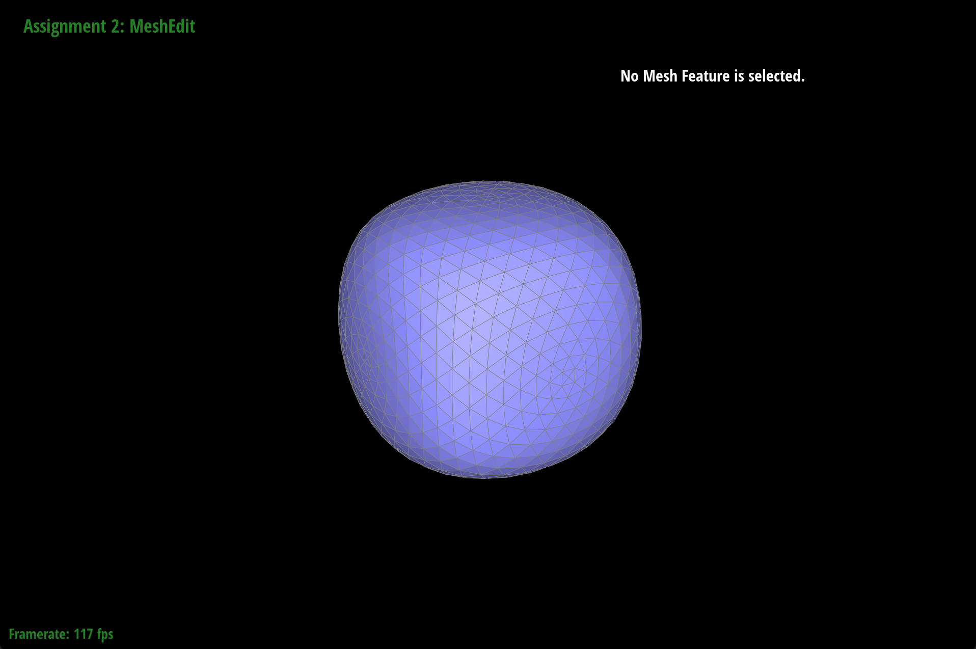
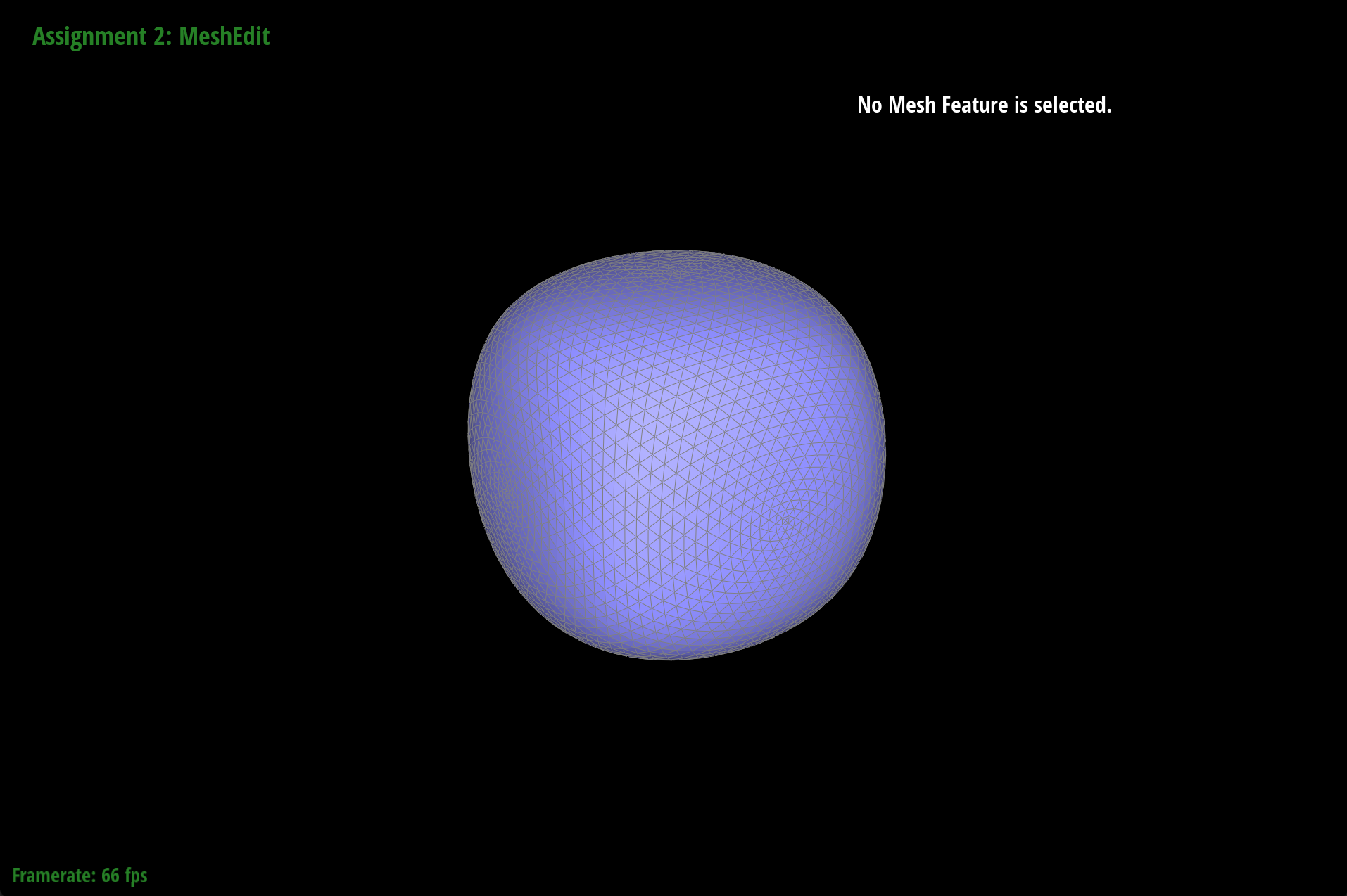
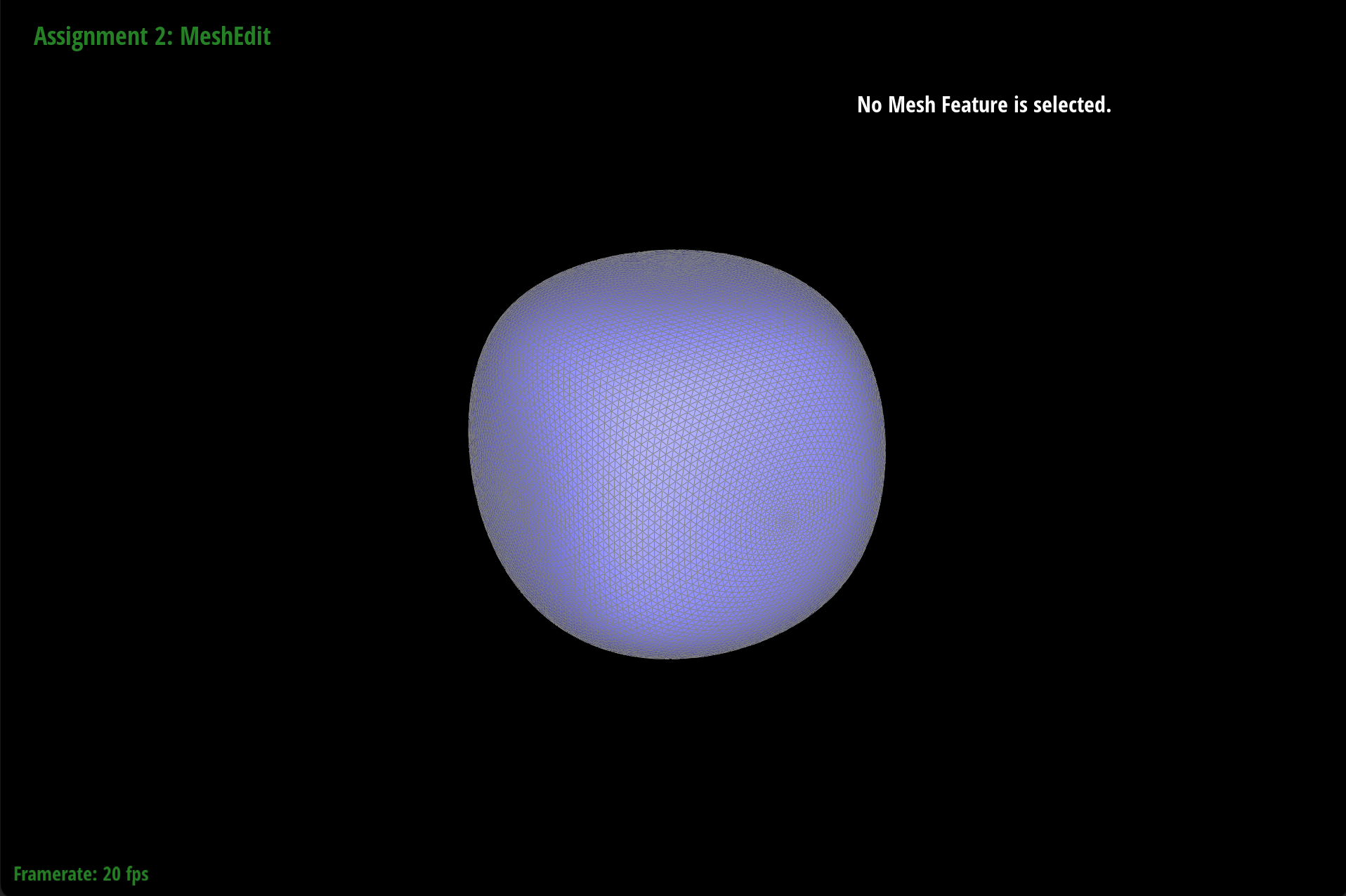
After loop subdivision, sharp corners and edges become smoother and rounded due to the addition of more edges. Sharp corners and edges seem to “disappear” or shrink into the mesh dramatically when we do loop subdivision.
|
|
|
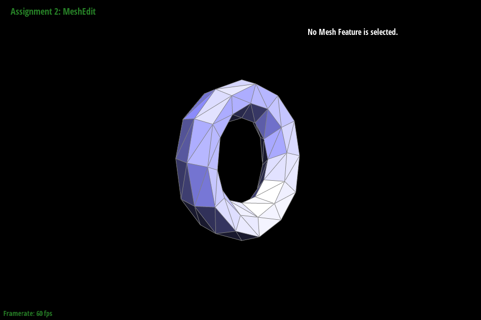
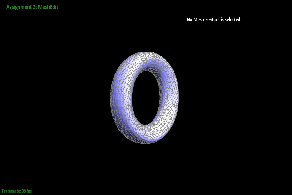
This is because on those sharp edges, the new vertex positions are calculated using neighbor vertex positions that are very “different” from each other which results in greater weighted averages (thus the big shrinking effect). We can indeed reduce this effect by pre-splitting some edges. Specifically, for example in the torus (../dae/torus/input.dae), if we split the outer flat faces, we get less shrinking in the edge when we upsample.
|
|
|
To pre-process the cube so that the cube subdivides symmetrically, we can split all edges on each flat face of the cube. The asymmetry from before was because the cube previously had only one edge splitting the face which resulted in asymmetrical subdivision because the face was asymmetrical to begin with. Our pre-processing (splitting all edges on each flat face of the cube) alleviates these effects because now we have two edges along each face (splits each face symmetrically) which should in turn subdivide symmetrically as well as we continue to upsample.
|
|
|
|
|
|