We implemented a simple rasterizer that draws triangles and uses various antialiasing algorithms such as supersampling, pixel sampling (nearest neighbor and bilinear interpolation), and level sampling (which was split into levels: level zero, the nearest level, and the weighted sum of adjacent levels of a continuous mipmap level). As a whole for this project, we have built a functional vector graphics renderer that can work with simplified SVG files and that has 6 different options/modes in total: two modes for image resampling (nearest and bilinear) and 3 modes for mipmap level resampling (level zero, nearest, and linear interpolation). Some interesting things we’ve learned from completing this project are that we don’t always need to recompute the full resolution image repeatedly when we want to apply textures by making use of mipmaps to store already computed textures of varying resolutions and applying those precomputed textures instead. It was interesting to learn that this technique is used in video games, which makes sense since video games already require a lot of computational power. We also learned that supersampling works better than expected and simply allows certain pixels to take on intermediate values to create a “blurred” effect and effectively remove jaggies. We really liked how making use of barycentric coordinates and abstracting math helped to replicate fascinating textures in our images. Overall, we just really enjoyed the visual aspect of our project and how implementing one concept at a time helped to create a fully functional rasterizer that can take in any SVG file. It was very satisfying and rewarding to see this project come together!
We first determined the bounding box parameters of any given triangle. Given the (x, y) coordinates of each triangle vertex, we found the maximum and minimum values of the set of x coordinates, as well as the maximum and minimum values of the set of y coordinates. The maximum x-coordinate served as the upper bound of the bounding box, and the minimum x-coordinate served as the lower bound of the bounding box in the x direction. The same logic applies to the maximum and minimum y-coordinates.
Then, we had two for loops: one that iterated through the x-values from the minimum x-coordinate to the maximum x-coordinate (inclusive), and one that iterated through the y-values from minimum y-coordinate to the maximum y-coordinate (inclusive). This ensures that we access all points within the bounding box of the triangle.
With each point (x,y), we sample whether the center of the pixel, (x + 0.5, y + 0.5), is inside the triangle using the three line test method introduced in Lecture 2, i.e. if (x + 0.5, y + 0.5) falls within the intersection of the three half planes given by line equations L0, L1, and L2, then the center of the pixel falls within the triangle. We sample this by seeing if L(x + 0.5, y + 0.5) >= 0 for all L0, L1, L2. If L(x + 0.5, y + 0.5) > 0, this means that the point is inside the edge, but we also consider cases where L(x + 0.5, y + 0.5) = 0, when the point falls on the edge, to be in the triangle.
One observation that we made was that the point-in-triangle model described in the slides applied to triangle vertices listed in a counterclockwise order. However, not all triangle vertices are given in this order. To address this, we implemented a test to see if the orientation of the triangle vertices was clockwise. If clockwise, we simply reversed the order of how we calculated dx_i for the line test (e.g., for counterclockwise orientation, dx_i = x_i - x_(i + 1), so for clockwise orientation, we did dx_i = x_i + 1 - x_i instead).
For supersampling, we applied the same logic for bounding boxes and the clockwise tests as task 1. However, this time, when we were iterating through all the points within the bounding box of the triangle using the for loops for x and y, we nested two more for loops. The two additional for loops each looped from 0 to sqrt(sample_rate) to ensure we sampled a total of sample_rate times per pixel. This would ensure our images are rasterized at a higher resolution before downsampling to the output resolution of the framebuffer later. Instead of adding 0.5 to each sample point within a pixel as in part 1, we derived an equation that would allow us to sample sample_rate times per pixel. The equation we used was (float) x + ((2 * (float) i + 1) / (2 * (float) N)) where x is the x-coordinate of the current pixel we’re sampling for and i is the i-th horizontal sample point we want to sample at for our pixel. Similarly, for y, we do (float) y + (2 * (float) j + 1) / (2 * (float) N), where y is the y-coordinate of the current pixel and j is the j-th vertical sample point we want to sample at for our pixel. Both i and j are maxed at square root of sample_rate since we want sqrt(sample_rate) x sqrt(sample_rate) = sample_rate samples for each pixel. Then, similar to task 1, we do the three line test to check if each subpixel is contained in the triangle. If it is, we write the color to the (sample_rate * (y * width + x) + k)-th index of the sample_buffer. The sample_buffer is a width * height matrix of Colors organized as a 1D vector, but is now size (width * height * sample rate). We do this because we want to scale the sample_buffer by sample_rate as we are sampling sample_rate times per pixel. Indexing the color to (sample_rate * (y * width + x) + k) allows us to track which sample point we are at at a given time (with k being the k-th number sample in the pixel).
Ultimately, we found supersampling to be useful because it allows for antialiasing (removal/reduction of jaggies) by making certain pixels (especially near edges of shapes) take on intermediate values.
|
|

|

|
|
For sample rate 1, we see a lot of jaggies and sometimes oddly connected/disconnected pixels. For sample rate 4 and especially sample rate 16, we do see blurring because now we are sampling multiple times per pixel (4 and 16 respectively) which allows us to calculate the average the color values of a pixel depending on if its samples fall within a triangle. We can observe that the antialiasing effects are stronger as the sampling rate increases.
|
|
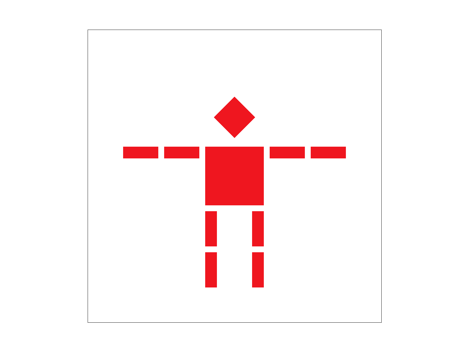
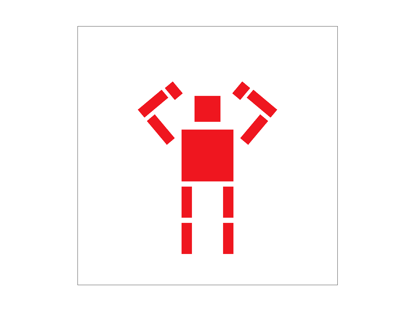
Our modified robot image depicts our robot trying to create a heart shape over its head using its arms (but it also looks like it's flexing really hard). To acheive this, we rotated and translated each pair of arm blocks (e.g. lower forearms, upper forearms) so that they could mirror each other. We also added in an additional hand block to close the heart shape, using matching angle rotations as the upper forearms. We also rotated the head back to an angle of 0.
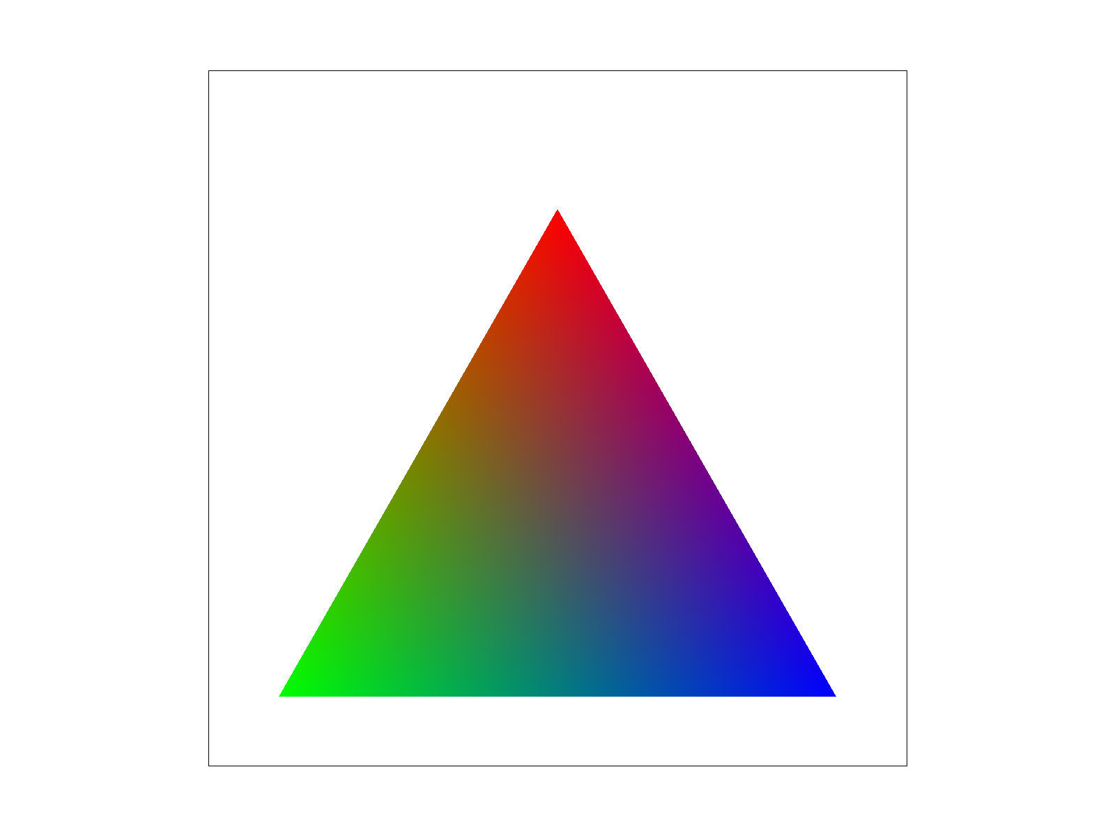
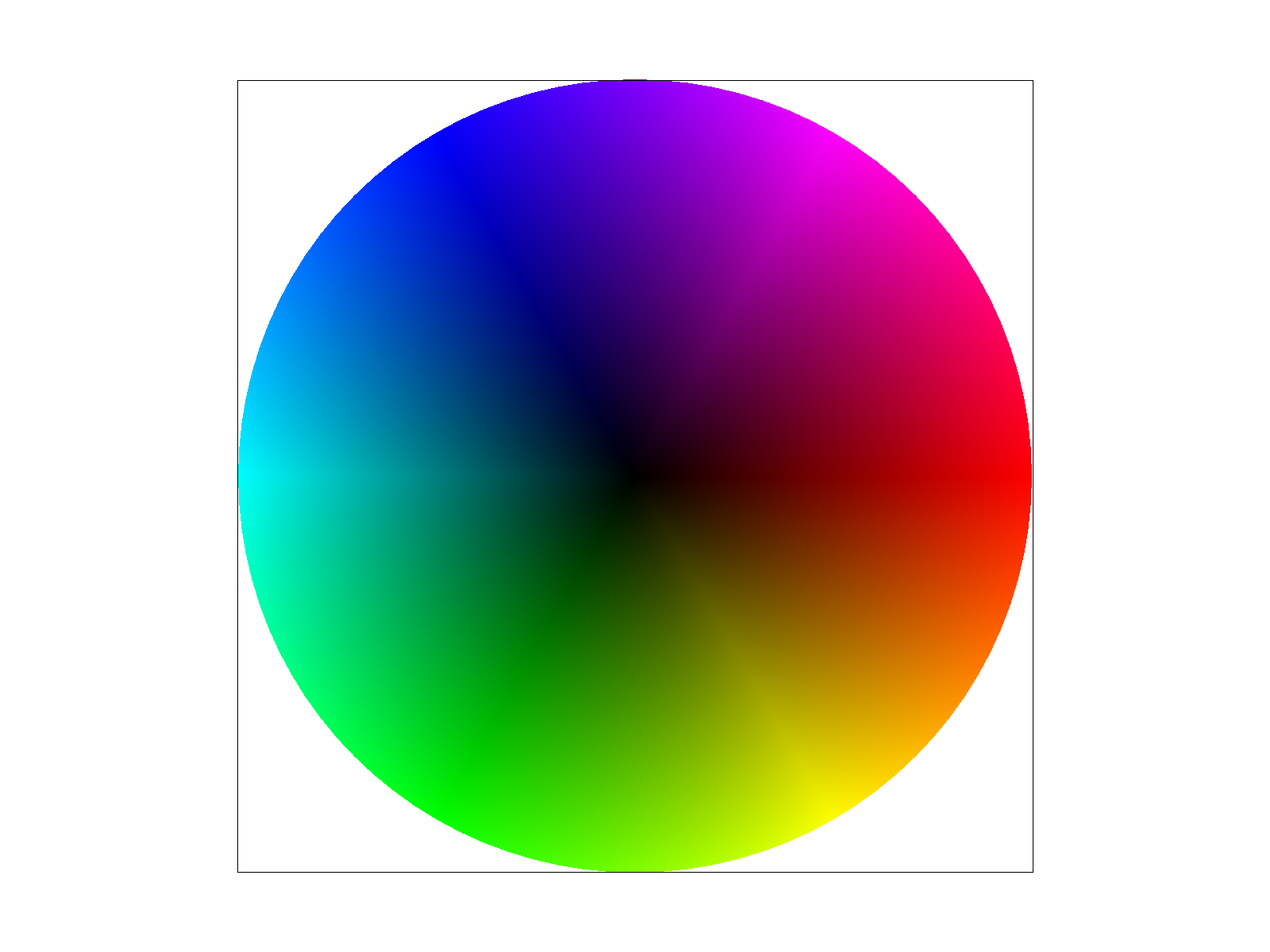
Barycentric coordinates are a coordinate system for triangles that allows us to linearly interpolate values at the triangle vertices (these values can be anything, e.g. texture coordinates, colors, normal vectors, etc.) and obtain smoothly varying values across the surface of the triangle.
|
|
To calculate the barycentric coordinates, which are represented by the weights (alpha, beta, gamma), we use triangle vertices A, B, and C. Then, given an (x, y) coordinate within the triangle, we solve the system of equations given to us by:
alpha + beta + gamma = 1
Alpha * A + beta * B + gamma * C = (x, y)
For our implementation, we stored the x and y components of vertices A, B, C in a 3 x 3 homogeneous matrix. Then, we multiplied the inverse of this matrix by the (x, y) coordinate represented as a 2D vector, which returns our barycentric weights of (alpha, beta, gamma).
Pixel sampling is a method of sampling for an image where we get a corresponding colored pixel back. In terms of texture mapping, pixel sampling is used to get a corresponding color of a texture pixel (pexel). Pixel sampling, at the highest resolution, is when there are many/multiple pixel samples at every texel sample, and at the lowest resolution, there is one pixel sample for many texel samples. Generally, pixel sampling works well for magnifying textures.
The two methods of pixel sampling we implement are nearest neighbor interpolation, where we consider the closest pixel and retrieve its corresponding color, and bilinear interpolation, where we take the colors of the surrounding pixels and apply linear interpolation to get a “middle” color back.
For nearest sampling, we rounded the given texture coordinates to the nearest texel at a given mipmap level. More specifically, given the coordinates of a texture pixel (u, v), we scaled the x and y coordinates by the mipmap level’s width and height minus 1 respectively. We then rounded both of the scaled coordinates and passed the scaled texture pixel coordinates as arguments in a call to get_texel, which returned a colored texel at the current mipmap level.
Bilinear sampling makes use of two linear interpolations horizontally and one vertical linear interpolation (accounting for the texture locations around the given sample texture value) in the final calculation of the texture color. Given texture coordinates (u, v), we again scaled each u and v coordinate (or x and y) by mip.width - 1 and mip.height - 1. We then calculated the top right, bottom left, top left, and bottom right texture sample location coordinates that were around our sample texture coordinate. Using these values, we retrieved the corresponding colors for each sample texel location using mip.get_texel(). We then performed linear interpolation (lerp) on the returned color values for each sample texture coordinate. Two of the lerps were for the horizontal “border”/nearest sample locations of the texture value to be sampled, and the other was for the vertical “border”/nearest sample location. In the end, after performing linear interpolation on all our 4 texture sample locations, we got a final color that was the result of applying linear interpolation on all 4 locations and their corresponding color values/texels. Finally, we call sample() in rasterize_textured_triangle() and write the corresponding pixel color to sample_buffer.
Comparing the two methods of pixel sampling, we understand that nearest sampling takes into account the one closest pixel to a given texture pixel in determining the color. Bilinear sampling takes into account the 4 surrounding texture sample locations around a given texture value we want to sample and performs linear interpolation on the surrounding colors. In the end, especially at lower resolution images, nearest sampling appears to produce sharper edges/jaggies in texture compared to bilinear sampling, which produces more of a “blurred” effect because it takes more colors into consideration (the surrounding texture sample locations).

|

|

|
|
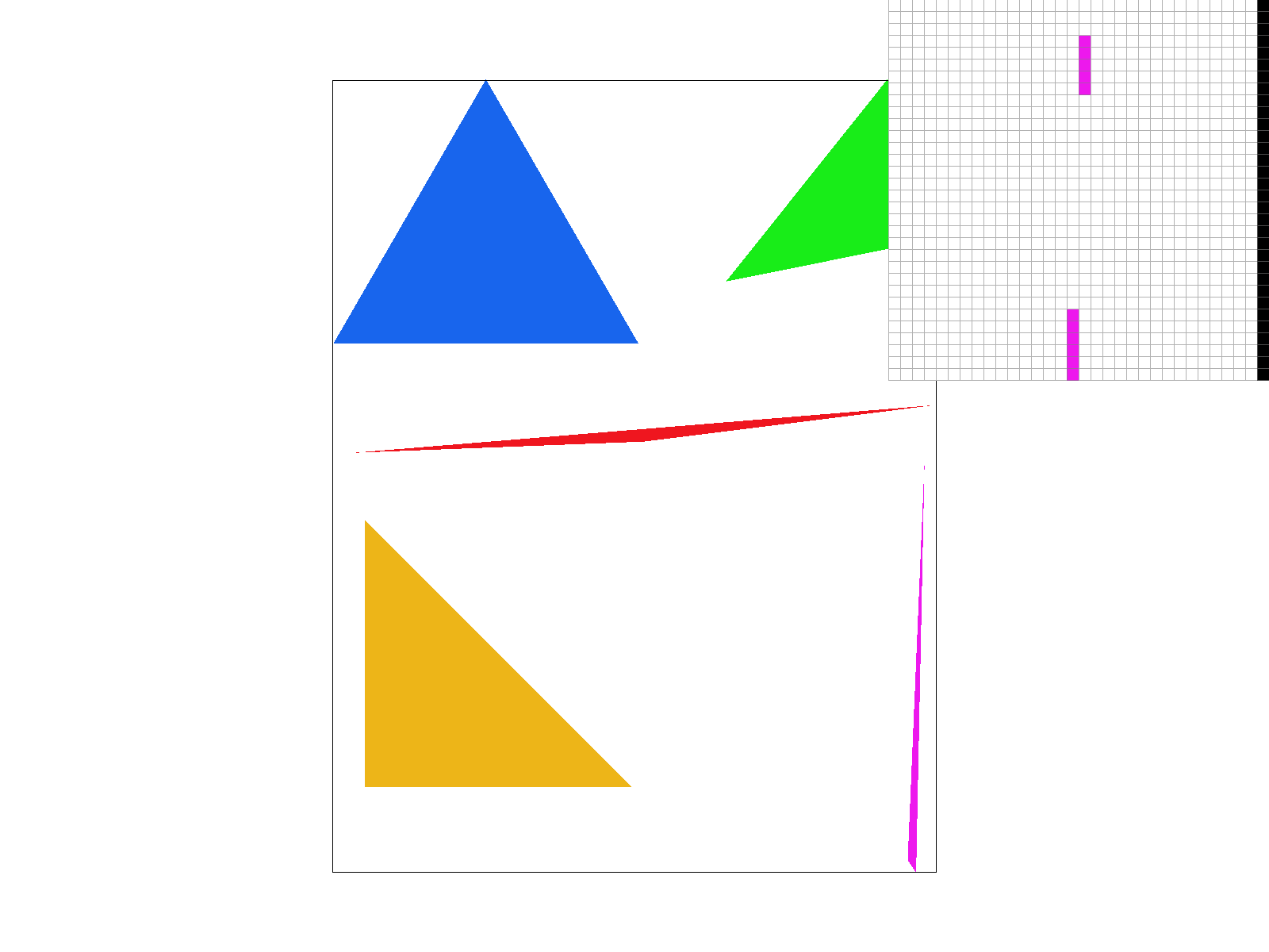
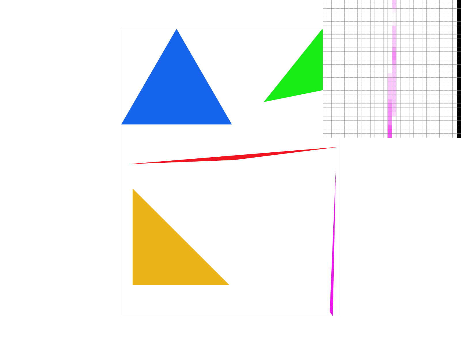
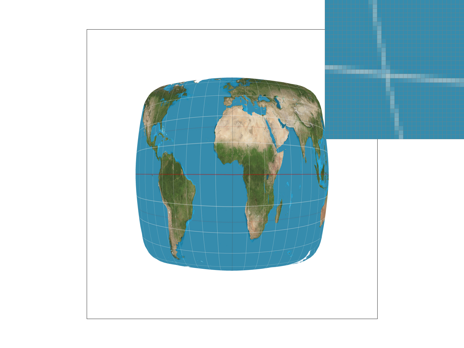
As seen in the images, bilinear sampling produces smoother looking lines than nearest sampling. For nearest sampling at 1 sample per pixel, the white grid lines look pixelated and disconnected, but for bilinear sampling at 1 sample per pixel, the lines look smoother and there is less aliasing. Meanwhile, the results for a nearest sampling rate at 16 samples per pixel and a bilinear sampling at 16 samples per pixel. These images show that bilinear sampling generally defeats nearest sample when working with low resolution images, but with high resolution images, the results of bilinear sampling and nearest sampling are similar.
There is a large difference between the two methods when we are working with low-resolution images because nearest sampling only takes into account the one closest pixel to a given texture pixel in determining the color. Bilinear sampling takes into account the 4 surrounding texture sample locations around a given texture value we want to sample and performs linear interpolation on the surrounding colors. This means nearest sampling appears to produce sharper edges/jaggies in texture compared to bilinear sampling, which produces more of a “blurred” effect because it takes more colors into consideration (the surrounding texture sample locations) and lower resolution images already have fewer pixels to work with which is why there is a larger effect.
The idea of level sampling is that we have different levels of sampling for a given image, where the lowest level (level 0) is the highest resolution and each successive level thereafter gets downsampled or has lower resolution. In the case of texture mapping, we apply the same idea where for each successive level we sample the texture file at a lower resolution and we store each successive lower resolution image. We used mipmaps, the stored filtered versions of a given texture of varying levels of resolution, and apply the textures to the closest image resolution of an image that needs a texture (for example, if an image is 64 by 64 pixels, we can just apply the closest mipmap in resolution to that image, such as a 62 by 62 pixel texture mipmap). The idea is that while not memory efficient (since we do need extra memory to store these extra textures), we can potentially save on computational power (faster rendering speeds) since we have a cache of mipmaps and can just query quicker than sampling the full resolution image again.
We implemented level sampling for texture mapping through three levels: level zero, the nearest level, and the weighted sum of adjacent levels of a continuous mipmap level. First, to retrieve our current mipmap level, we implemented get_level by taking the max(sqrt((du/dx)^2 + (dv/dx)^2), sqrt((du/dy)^2 + (dv/dy)^2)) and taking the log base 2 of the resulting max value to get mipmap level D. We got du/dx by doing (sp.p_dx_uv.x - sp.p_uv.x) and scaling it by the width, dv/dx by doing (sp.p_dx_uv.y - sp.p_uv.y) scaled by height, du/dy through (sp.p_dy_uv.x - sp.p_uv.x) scaled by width, and dv/dy through (sp.p_dy_uv.y - sp.p_uv.y) and scaled by height.
We also checked if D was less than 0, in which case we simply return 0 for the level. If D was greater than the mipmap size-1, then we returned the mipmap size-1 since that is the maximum mipmap level. If the level was zero, we simply passed in 0 for the level argument in sample_nearest and sample_bilinear, our pixel sampling methods which we implemented for every level sampling method. For sample_nearest at mipmap level 0, we scaled the corresponding uv coordinate by the mipmap’s width-1 and height-1 before rounding both u and v and retrieving the texel of the uv coordinate. For sample_bilinear, we similarly scaled the uv coordinates but instead of rounding to the nearest texel coordinate, we calculated the 4 nearest sample locations using floor and ceil before retrieving the corresponding colors/texels and performing linear interpolation on those 4 retrieved colors (which we did in task 5). For nearest level sampling, we rounded our level (which we got using get_level(sp)) to the nearest level and passed our level into sample_nearest and sample_bilinear, similar to what we did for level 0 (except this time we have a different level). For the weighted sum of adjacent levels of a continuous level (when sp.lsm is L_LINEAR), we retrieved the current level using get_level, then we took the floor of the level to get the lower adjacent value of the continuous level, and ceil to get the upper adjacent level. We then subtracted the upper level from the current level to get the lower weight, and subtracted the lower weight from 1 to get the upper weight. Finally, to get our weighted level that we would pass into sample_nearest and sample_bilinear, we did (lower_weight * lower) + (upper_weight * upper). In rasterize_textured_triangle(), we assigned our calculated barycentric differentials to attributes in the SampleParams struct. Our structure was similar to rasterize_interpolated_color_triangle with the clockwise/counterclockwise tests and for loops over every pixel as well as the for loops that went over the subpixels within a pixel (for antialiasing) and line tests, but this time we also calculated the barycentric coordinates for (x, y), (x+1, y), and (x, y + 1) and computed their respective texture coordinates. We then got the corresponding texel and wrote to the sample_buffer.
One problem we encountered in our implementation of level sampling was when the mipmap level was a continuous number and we needed to take a weighted sum of the adjacent levels. At first, we were really stuck because we overcomplicated this and thought we needed to account for cases where one weight was greater than the other. We thought about putting some if statements in to account for making sure the weight for the closest adjacent level was higher than the adjacent level that was further from the actual level, however, we realized after going through some examples and drawing the different cases out that it didn’t matter which weight was greater because the weighted sum would naturally account for which weight was greater based on the way we wrote our weighted level calculation (weighted_level = (lower_weight * lower) + (upper_weight * upper), where lower is the floor of the actual level and upper is the ceil of the actual level, and lower_weight is calculated with the upper level minus the current level and the upper_weight was calculated based on 1 minus the lower_weight). As such, we did not need extra if statements.

|

|

|

|

|
|
Among the three sampling techniques (pixel sampling, level sampling, and supersampling), we were able to see that pixel sampling and level sampling are faster than supersampling, whereas supersampling a high number of samples per pixel results in stronger antialiasing power, but requires more memory usage since it needs more storage for resizing the buffer to accommodate more samples of a higher resolution image.