CS184/284A Spring 2025 Homework 3 Write-Up

Link to webpage: https://cal-cs184-student.github.io/hw-webpages-stephen_webpage/hw3/index.html Link to GitHub repository: https://github.com/cal-cs184-student/sp25-hw3-stephen_hw3

Overview

In this homework, we implemented a path tracer to render scenes with realistic, physically accurate lighting. This computation is very expensive, so we implemented methods like BVH and adaptive sampling to speed up our rendering. We tried various sampling methods and implemented global illumination to better capture lighting details.

Part 1: Ray Generation and Scene Intersection

At a high level, a path tracer generates traces rays from the camera into the scene and determines which objects they intersect. Ray generation begins in the image space where we generate some number of rays for each pixel. We can then transform this location in the image space to the camera space, compute the direction, and finally transform the ray to world space.

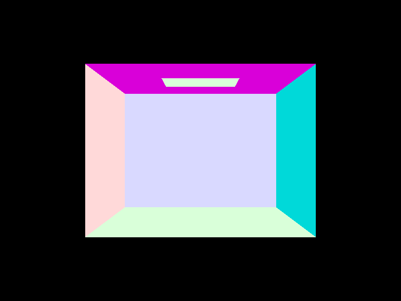
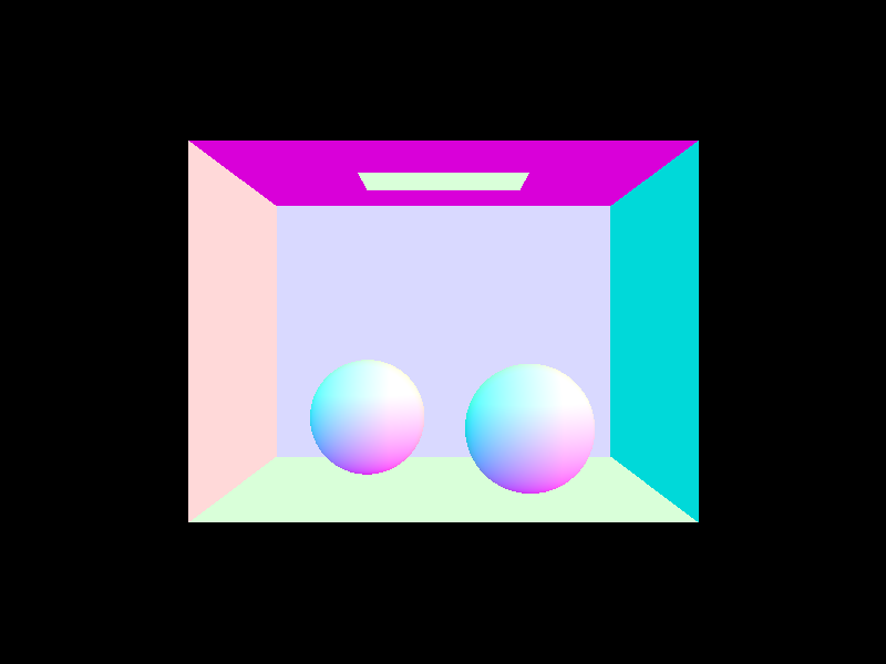
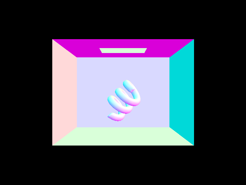
Now that we have generated valid rays, we want to see how this ray interacts with the objects in the scene. To figure out if a ray has hit something as it traverses, we loop through all scene objects and test for intersection. We'll walk through how this works for traingles as an example. For triangles, we can use the Moller-Trumbore algorithm. In this algorithm, after we calculate the edges and points of the triagnel shifted in barycentric coordinates, we can compute the parameters t, b1, and b2. Now, as long as t >= 0, 0 <= b1, 0 <= b2 <= 1, 0 <= 1 - b1 - b2 <= 1, all hold true, there is a valid intersection. When a ray intersects any object, like the triangles we just described for example, we save some data such as normal and BSDF that we can use to determine what color this intersection contributed to the pixel. Now we can render some simple scenes with normal shading.

Part 2: Bounding Volume Hierarchy

In this next section, we implemented a bounding volume hierarchy (BVH) to help accelerate the computation of intersections compared to naively checking all the primitives for intersection. We construct our BVH by starting with a minimum bounding box that contains all the primitives. We then check to see if the number of primitives in the scene is less than or equal to a max_leaf_size parameter, in which case the node is complete and we are done constructing. If this is not the case, we split the bounding box by choosing the axis with the greatest range of values and splitting on the centroid of the primitives. We recursively call this on the resulting 2 halves until completion.

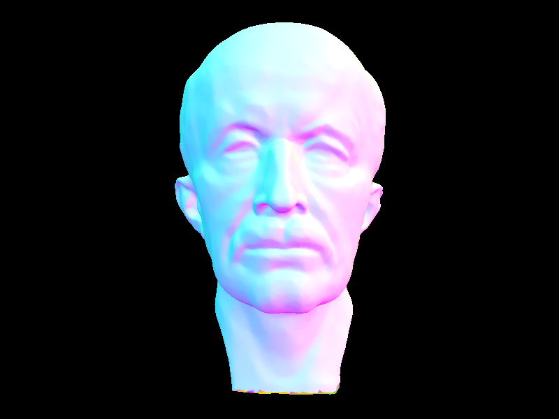
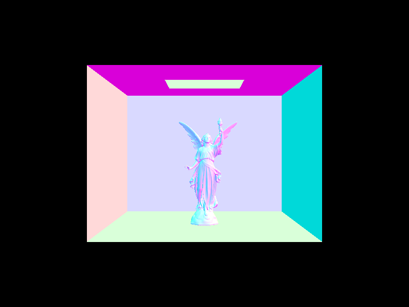
With BVH now implemented complex scenes with a lot of primitives could now be rendered in a reasonable amount of time. As recommended, Maxplanck which has on the order of 10,000 triangles saw a ~270x speed-up and CBlucy which has on the order of 100,000 triangles saw ~590x speed-up. This demonstrates that the BVH implementation scales better as the scenes get more complex. Here's some data to demonstrate this:

Cow.dae: ~32s -> ~0.4s Maxplanck.dae: ~387s -> ~1.4s CBlucy.dae: ~1475s -> ~2.5s

Here's what the Maxplanck and CBLucy scenes look like:

Part 3: Direct Illumination

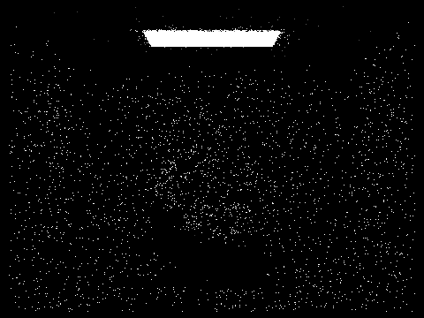
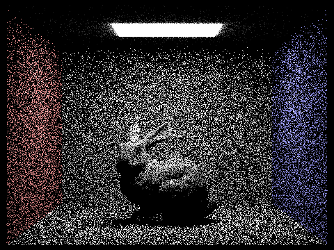
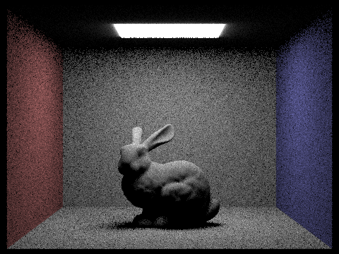
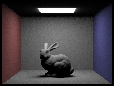
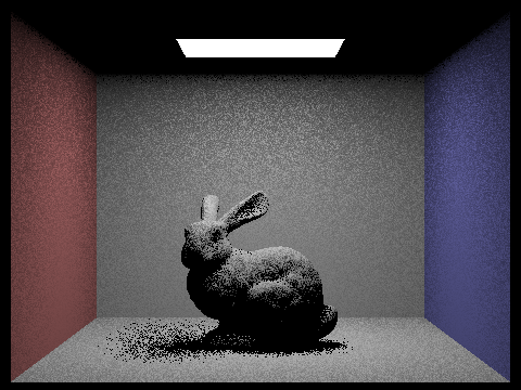
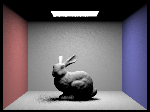
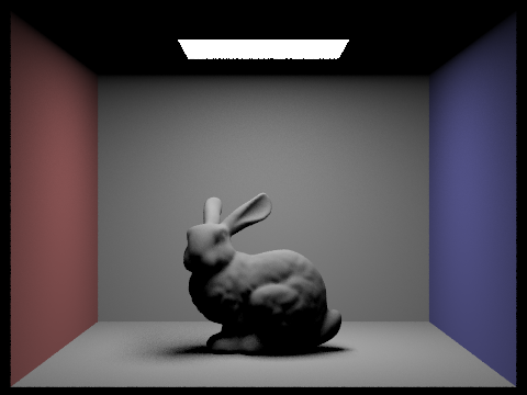
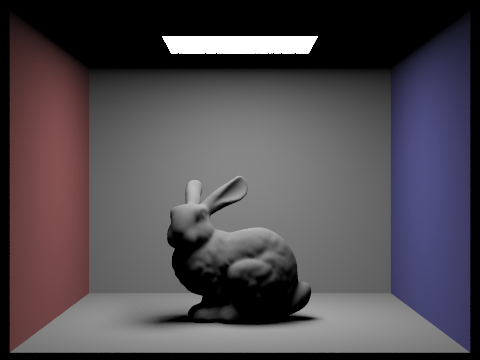
In this section we implement direct illumination, meaning light rays with 0 bounces (coming directly from a light source to the camera) and 1 bounce (light that bounces off a primitive in the scene directly into the camera). We implemented this in 2 ways: uniform hemisphere sampling and importance sampling. For uniform hemisphere sampling, when a ray intersects a primitive at some point in our scene, we take some number of samples uniformly around the hemisphere above the point to see if it intersects a light source. If one of these samples hit a light sources, it contributes to the ray hit. This method can produce very noisy, grainy renders without enough samples, because you might not hit a light source even if it's possible. This leads into importance sampling, the second method we implemented here. For importance sampling, we leverage the fact that we know where all the lights in the scene are, and only sample in that direction with shadow rays. If the shadow ray manages to hit the light, it contributes, and if it hits some other object in the scene first, it does not contribute. This greatly improves the visual quality of our renders without having to crank up our sampling parameters to unreasonable levels.

Here's a comparison of these two methods side-by-side with a wide range of sampling parameters. We have uniform hemisphere sampling on the top, and the analogous iportance sampling render on the bottom.

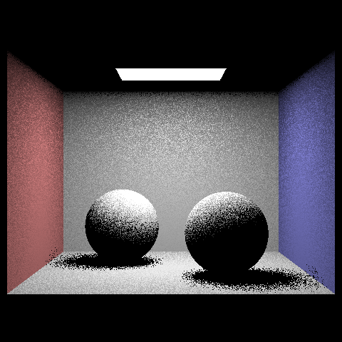
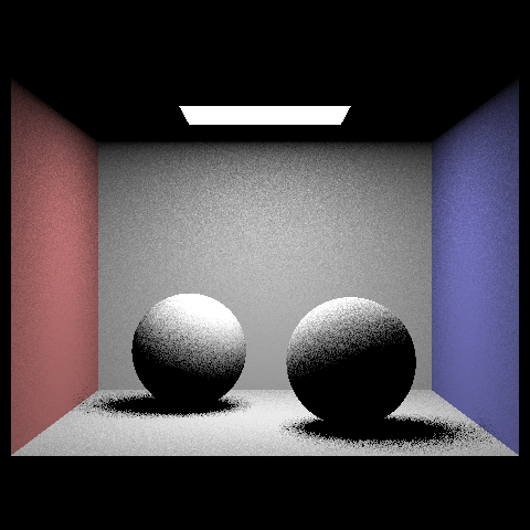
Here's the spheres scene with varying numbers of light rays, while keeping the number of samples we take constant. If we look at the soft shadows, we can see that increasing the number of light rays dramatically decreases the amount of noise, even when we are using importance sampling.

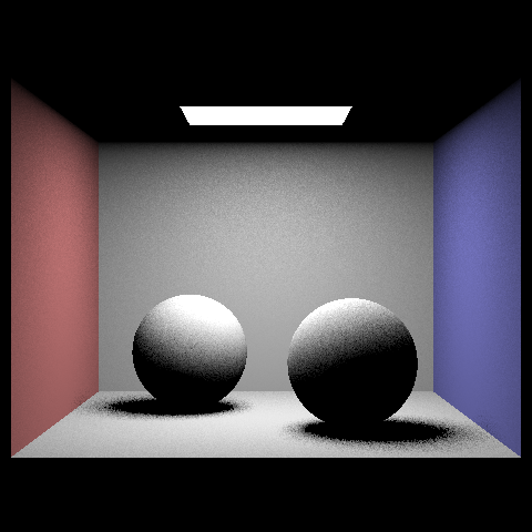
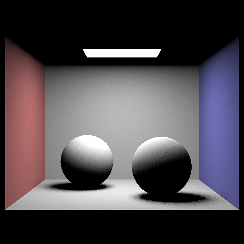
Part 4: Global Illumination

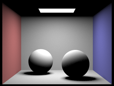
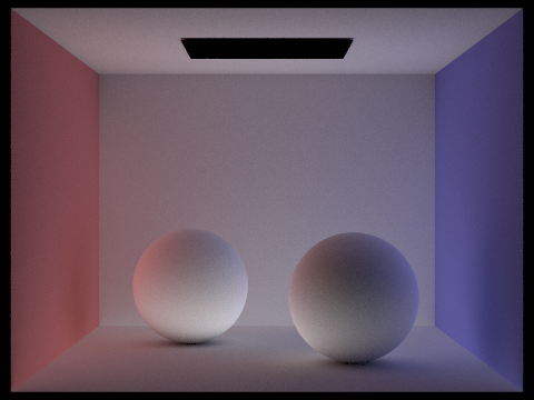
In this section we implement global illumination to enable more rich visual qualities in our scenes. To do this we need to account for indirect lighting, where we are now integrating the 2nd, and the 3rd, and the 4th, etc. bounces that the light takes. We do this by recursively calling at_least_one_bounce_radiance to accumulate light as it does these successive bounces throughout the scene. We pass in a max_ray_depth parameter, that we decrement throughout this recursion until we reach a base case of the final bounce that's allowed. When we combine this with the 0 bounce case from the previous section, we get our final global illumination results. Here's a couple of scenes that we've rendered with global illumination enabled:

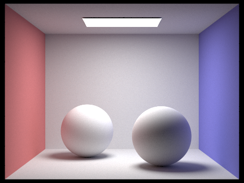
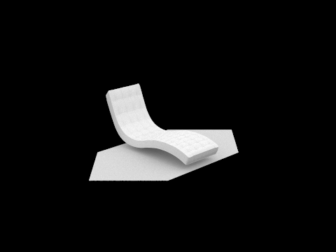
Here's a decompisition of the sphere scene with only the direct lighting on the left and only the indirect lighting on the right:

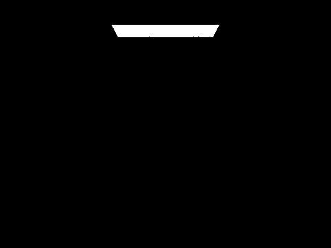
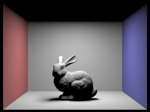
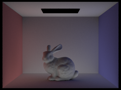
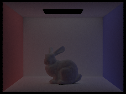
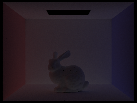
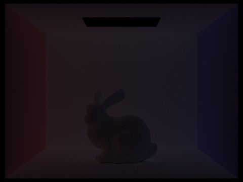
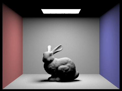
Now let's look at the bunny scene. We have functionality to not accumulate the light as it bounces. That is when this feature is enabled, we only render the light returned by the last bounce. Below we show this for varying maximum numbers of bounces.

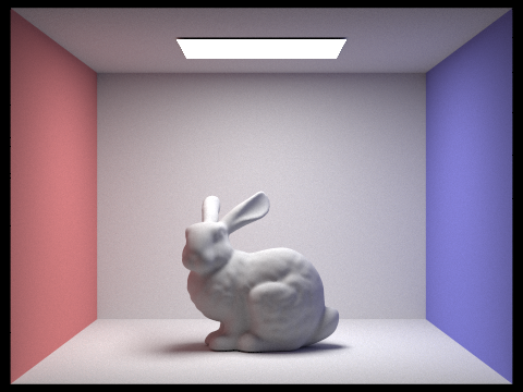
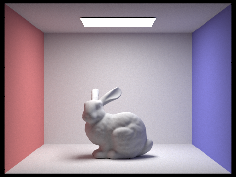
Here's what this looks like if we were to accumulate the bounces instead:

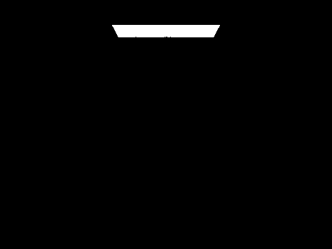
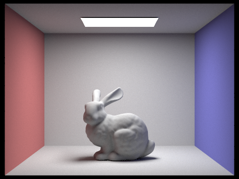
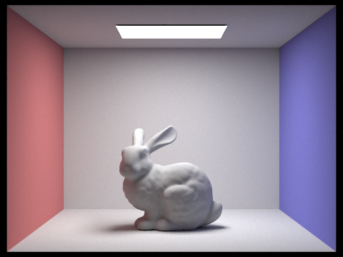
If we take a look particularly at the 2nd and 3rd bounces, we can see that the 2nd bounce enables for lighting on the underside of objects such as the underside of the bunny and the ceiling in the scene. With the 3rd bounce we can start to see more smooth color bleeding. When compared to traditional rendering methods like rasterization, we can capture these realistic, physical effects in our final render in a way that rasterization does not capture.

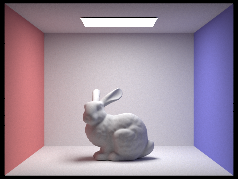
We also implemented russian roulette to get an unbiased method for reducing computation time. Our renders after implementing this are shown below. We can see that the visual quality is pretty much the same, but we can now handle much larger numbers of bounces like the 100 bounce case we show without having ridiculously long render times.

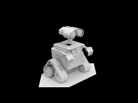
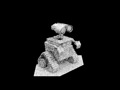
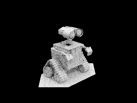
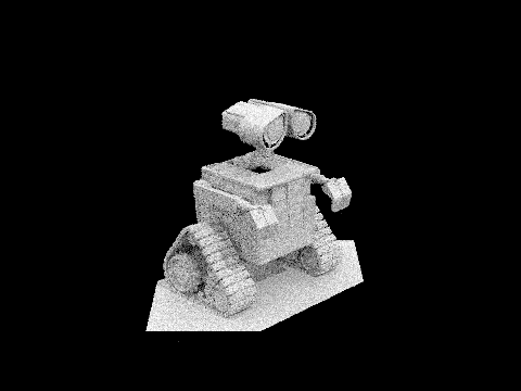
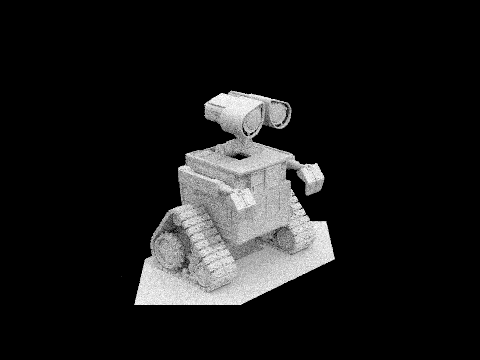
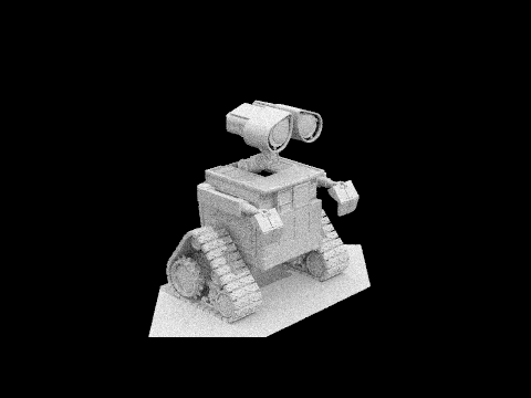
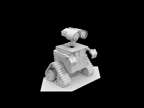
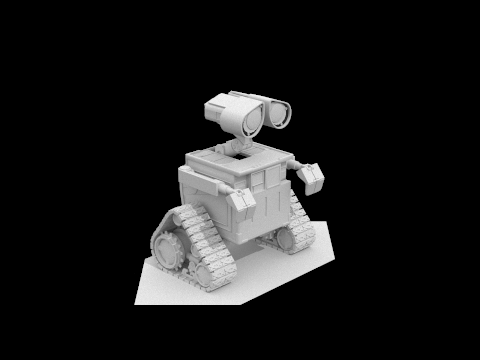
Finally let's look at the wall-e scene with varying sample-per-pixel rates:

Part 5: Adaptive Sampling

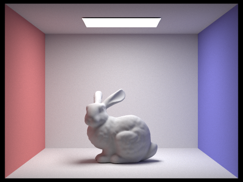
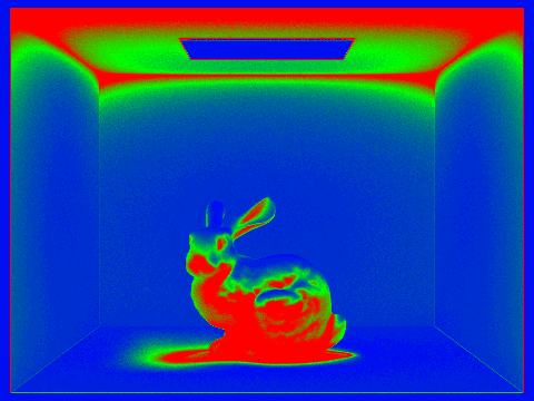
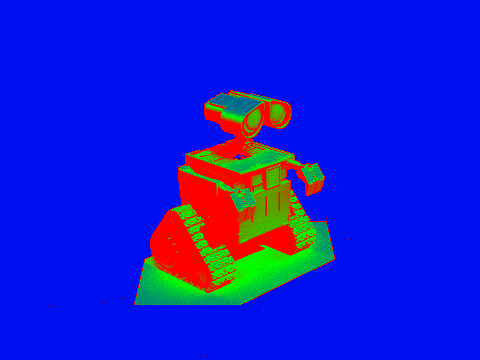
The final feature that we implemented here was adaptive sampling. This is a simple method for speeding up our renders by tracking how much a pixel value is changing from the additional sample. Once the pixel isn't really changing that much, that means that it's converged to the value that we want, and it's safe to stop sampling. We create a confidence interval such that we are 95% certain that the pixel is done. If the pixel is done, we simply break out of our sampling loop and stop sampling for that pixel. Here's a couple of scenes with a heat map of each pixel's needed sampling rate and the actual render that was made: