CS184/284A Spring 2025 Homework 2: Mesh-Edit

Link to webpage: https://cal-cs184-student.github.io/hw-webpages-stephen_webpage/hw2/index.html
Link to GitHub repository: https://github.com/cal-cs184-student/sp25-hw2-stephen_hw2

Overview

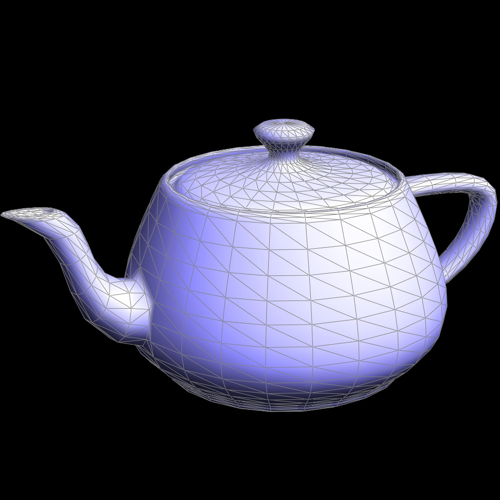
In this assignment we focused on geometric modelling methods that we discussed during lecture, particularly Bezeier curves and surfaces using the de Casteljau algorithm, and manipulating half-edge meshes culminating in Loop subdivision of meshes.

Section I: Bezier Curves and Surfaces

Part 1: Bezier curves with 1D de Casteljau subdivision

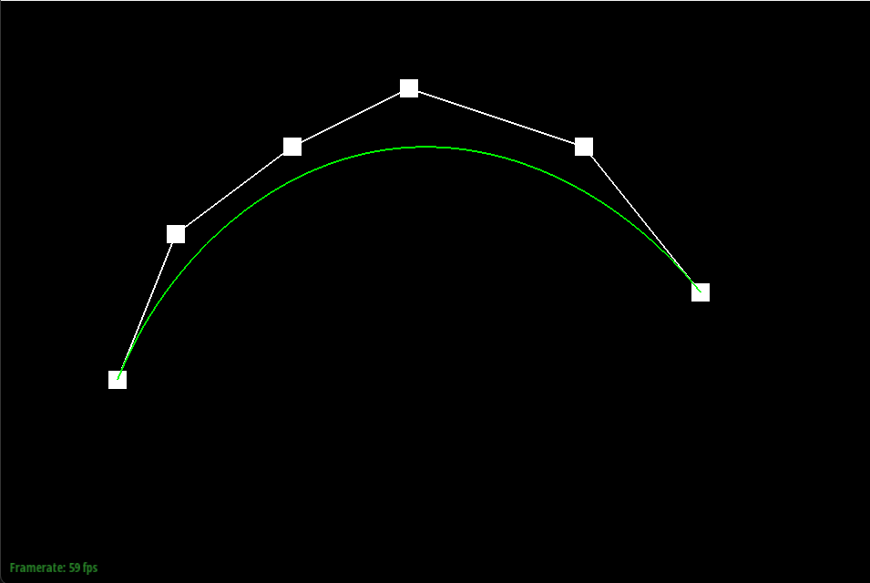
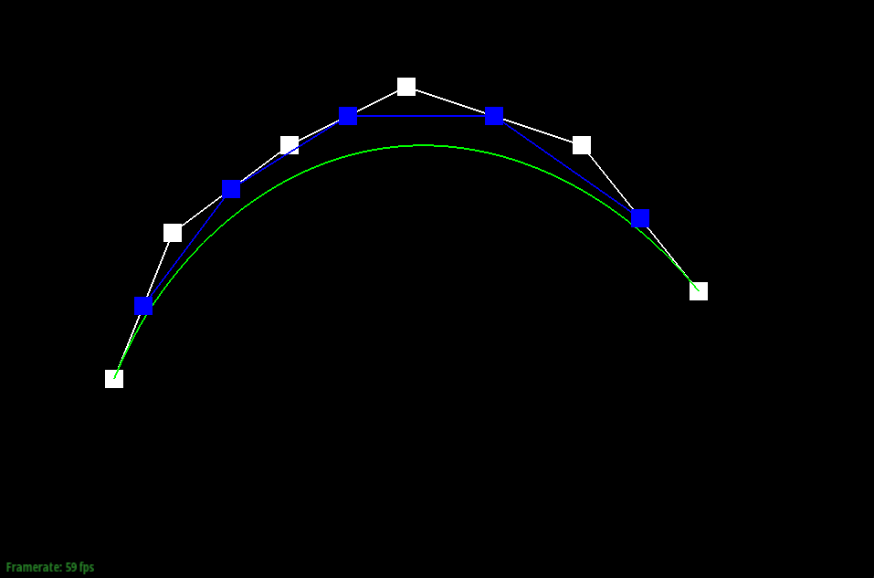
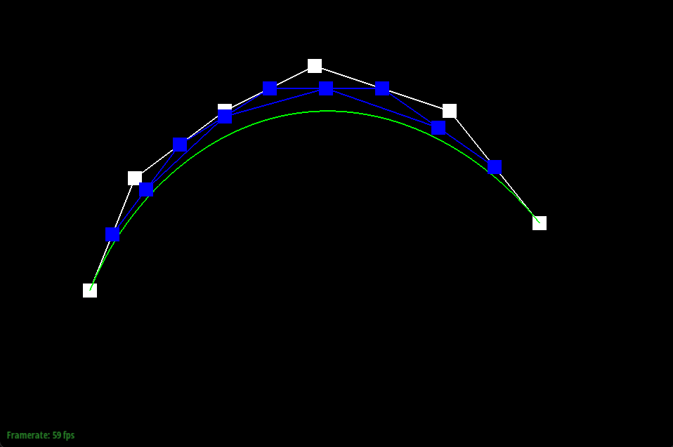
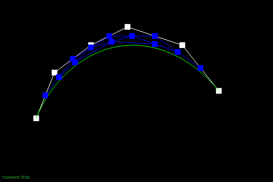
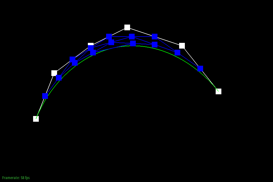
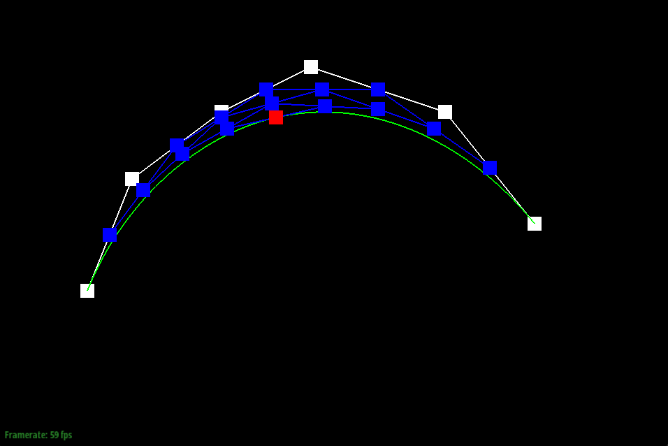
Bezier curves are parametric curves that are frequently used in computer graphics, animation, and geometric modeling. An individual curve is defined by a set of control points, which are used to determine the curve's shape. The curve smoothly interpolates between the first and last control points while being influenced by the intermediate ones. De Casteljau's algorithm is a method for forming Bezier curves by repeatedly applying linear interpolation to control points. Specifically, at each level, given some interpolation ratio t, each pair of the n control points are linear interpolated to find n - 1 new control points for the next level of computation. This process repeats until there is only 1 point left, and this is the point on the Bezier curve.

Here's an example of the De Casteljau algorithm at work. You can see how at each level we compute n - 1 new control points until we end up with just the one red square point on the Bezier curve at level 5

My implementation of De Casteljau's algorithm allows the user to do this level by level. Every time the user hits the E key, we evaluate one step of De Casteljau's algorithm, that is we apply linear interpolation to every pair of input points and output the resulting points. The user can can keep doing this to see what happens level by level as demonstrated in Figure 1 until we reach the base case of 1 point where the algorithm concludes with a point on the Bezier curve.

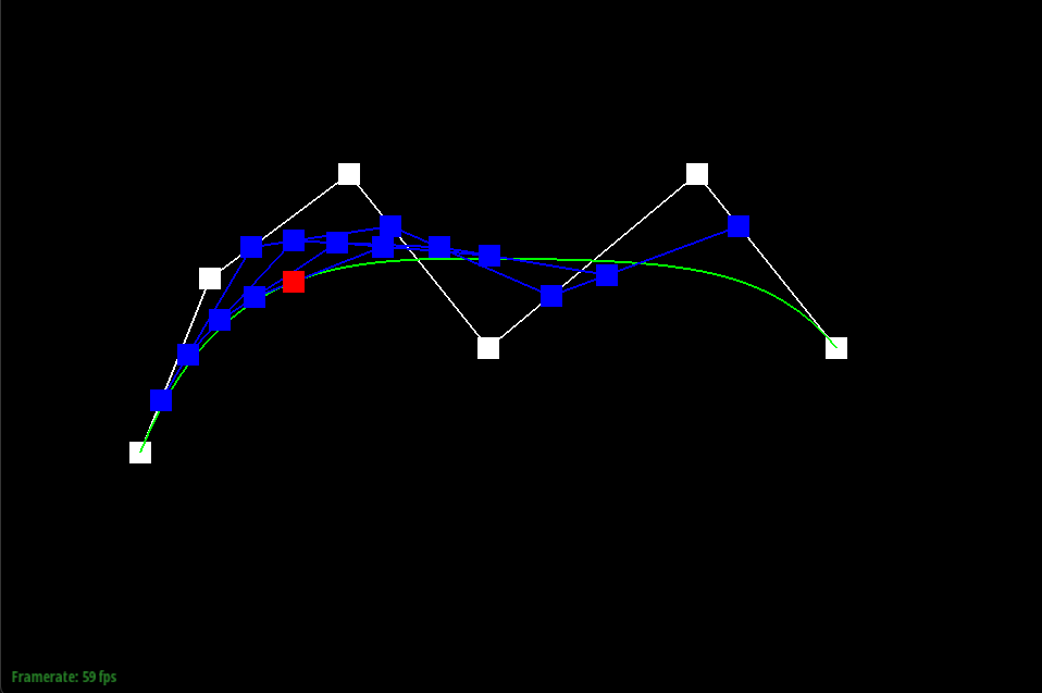
Part 2: Bezier surfaces with separable 1D de Casteljau

We can extend De Casteljau's algorithm to create Bezier surfaces as well. First we find the Bezier curves that represent row of control points just like in the previous part parameterized by u. We then the corresponding control points and parameterize by v that roughly lie along a column. We then apply the recursive step again to evaluate the single final point on the Bezeier surface parameterized by u, v.

My implementation can be broken down in the following functions:

evaluateStep(): Performs one step of De Casteljau’s algorithm for a vector of control points.

evaluate1D(): Calls evaluateStep() repeatedly until only one point remains to compute a single Bezier curve in 1-dimension.

evaluate(): Computes the Bezier surface point using evaluate1D() along two dimensions parameterizing by u, v.

Section II: Triangle Meshes and Half-Edge Data Structure

Part 3: Area-weighted vertex normals

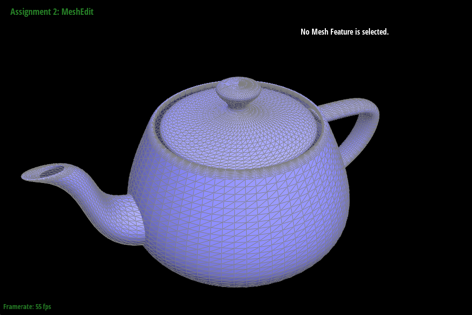
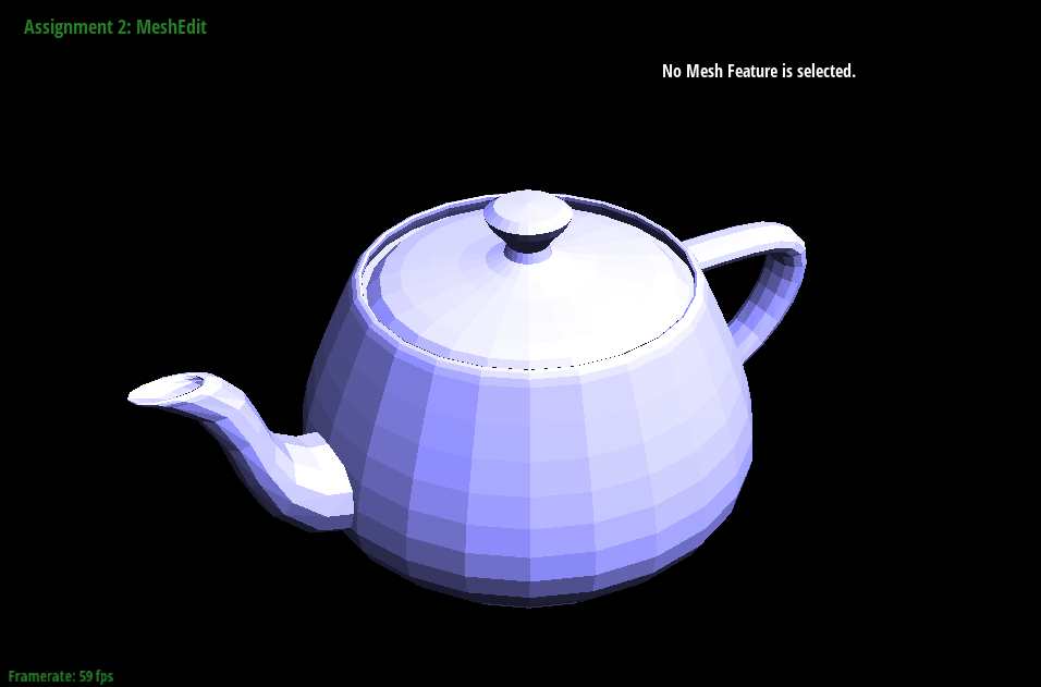
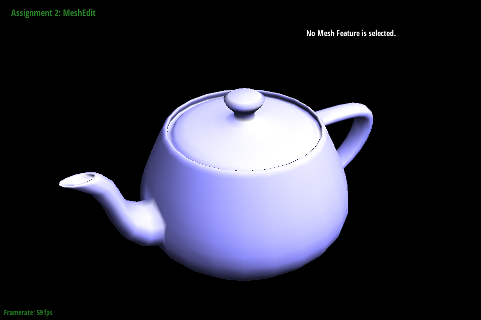
I implemented the area-weighted vertex normals by iterating over all faces adjacent to a given vertex. For each adjacent face, I found its normal vector and its area. I then computed weighted average of these normal vectors, weighted by the area of its face. This enables us to have Phong shading, which we compare below in Figure 4 against flat shading

Part 4: Edge flip

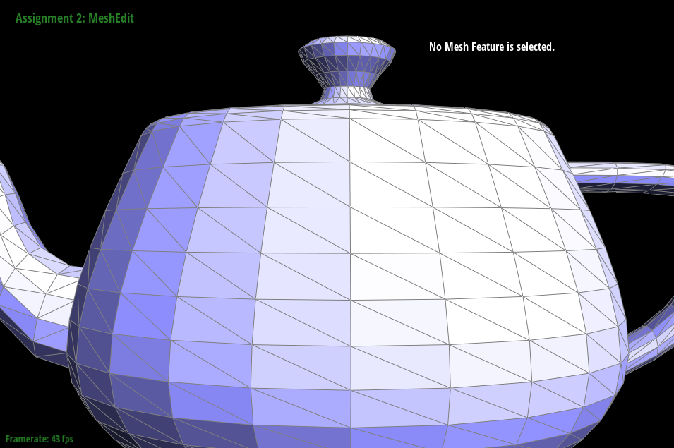
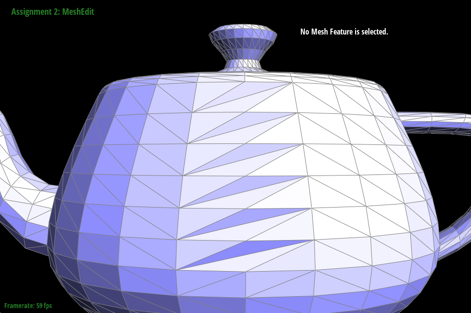
In this part we implemented edge flips. This is a local remeshing algorithm that given a pair of triangles, takes their shared edge and flips it such that the shared edge now connects the previously unconnected vertices. I found that drawing a picture was helpful in implementing this operation, and that it was fairly straightforward as long as I kept track of all the data structures that I was handling in the diagram. Below is an example of how this works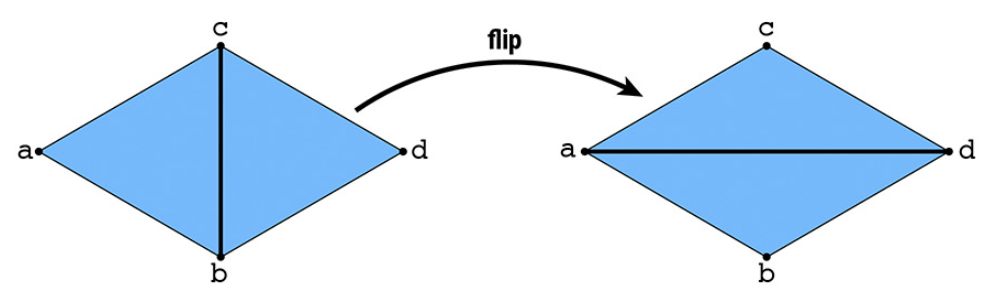

Taking the input edge, (b, c) in Figure 5, I traversed both triangles to identify the 4 vertices, 5 edges, 10 half-edges, and 2 faces that I was working with. I then modified the pointers for the edge (b, c) that got flipped to connect (a, d) instead. I then appropriately reassigned the pointers to the vertices, edges, half-edges, and faces that I had identified earlier to match the new topology. Here's an example of this edge flipping in action:

Part 5: Edge split

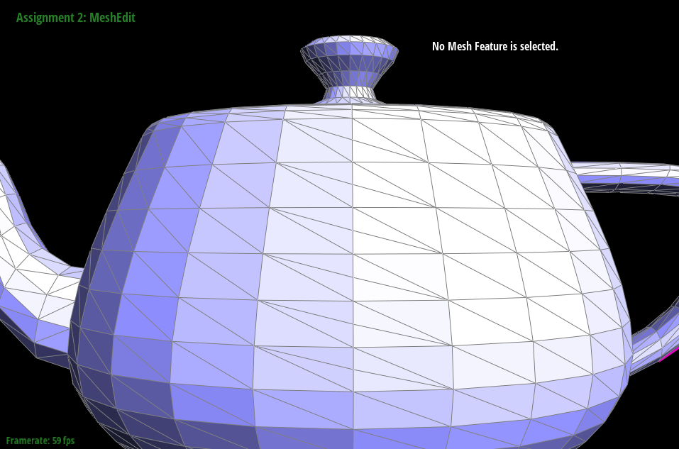
In this part we implemented edge splitting, which is another local remeshing operation. To perform an edge split, given a pair of triangles, we split the edge that they share at its midpoint and connect that midpoint to the opposite vertex of each triangle. This operation was a little more involved than edge flipping since we are actually adding new elements to our mesh data structure here. Once again, I found that drawing a diagram to track all the moving parts was very helpful. Below is an example of an edge slip in action: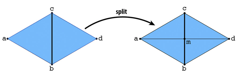

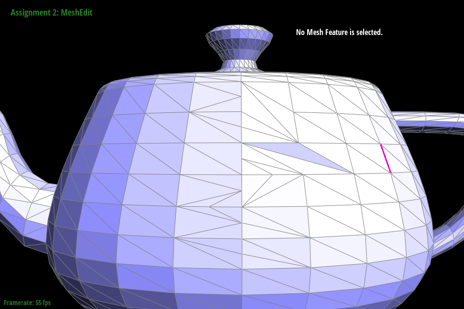
Once again takin the input edge (b, c), we want to traverse both of the triangles to to identify the original 4 vertices, 5 edges, 10 half-edges, and 2 faces that I was working with. In the split operation we are adding 1 new vertex, 3 new edges, 6 new half-edges, and 2 new faces. I begin by finding the midpoint of (b, c) which is the new vertex that we are adding. I then created the 3 new edges (a, m), (m, c), and (m, d) in Figure 7 along with their corresponding half-edges while ensuring proper orientation. The original edge (b, c) gets modified to represent (b, m) in Figure 7. Finally I create 2 new faces that correspond to the triangles (a, m , c) and (d, c, m), while the original faces correspond to their respective half-edges from the original edge (b, c). Having created all these new elements, I now assign and reassign pointers to elements accordingly to the new topology. A few notes on some interesting bugs that I encountered. The weirdest issue that I ran into while implementing this part was an access exception that was being thrown at seemingly random times after performing an edge split. I could see that my edge split happened, and it visually looked like what I would expect to see, but after some time sometimes almost immediately and other times after around 10 seconds, my program would crash with an illegal access exception at inline Vertex* HalfedgeElement::getVertex ( void ) { return dynamic_cast ( this ); }. After unsuccessfully trying to trace this call back, I took a step back and looked through all the data structures that we were providing to make sure that I was initializing everything properly. Weirdly enough I found that I had forgotten to set the Edge for each of the new half-edges, which was pretty unituitive given where my program would crash, but after doing this everything ran fine!

Part 6: Loop subdivision for mesh upsampling

I implemented Loop subdivision following the the suggested implementation in the starter code:

1. Compute the new positions for all vertices using the Loop subdivision rule and store this for later

2. Compute new positions for all the edges

3. Split the edges of the original mesh and mark new edges as new

4. Flip any of the new edges that connect old and new vertices

5. Copy the new vertex positions that we stored in step 1 into final positions

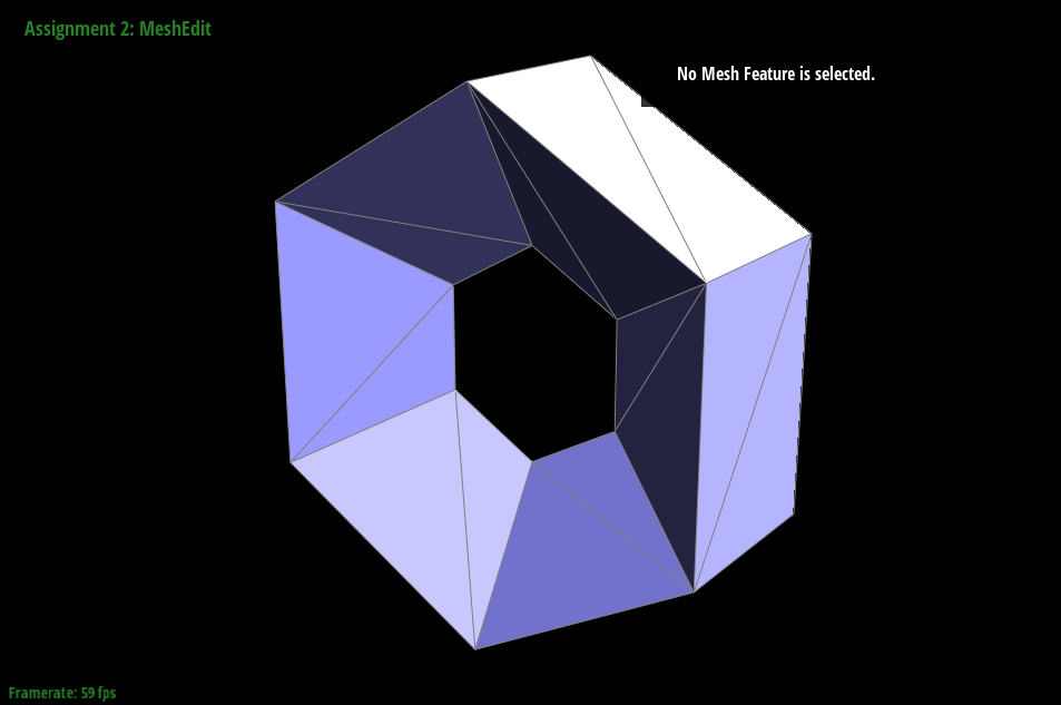
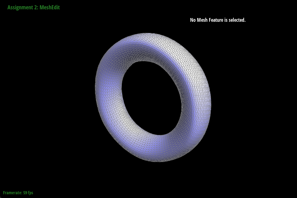
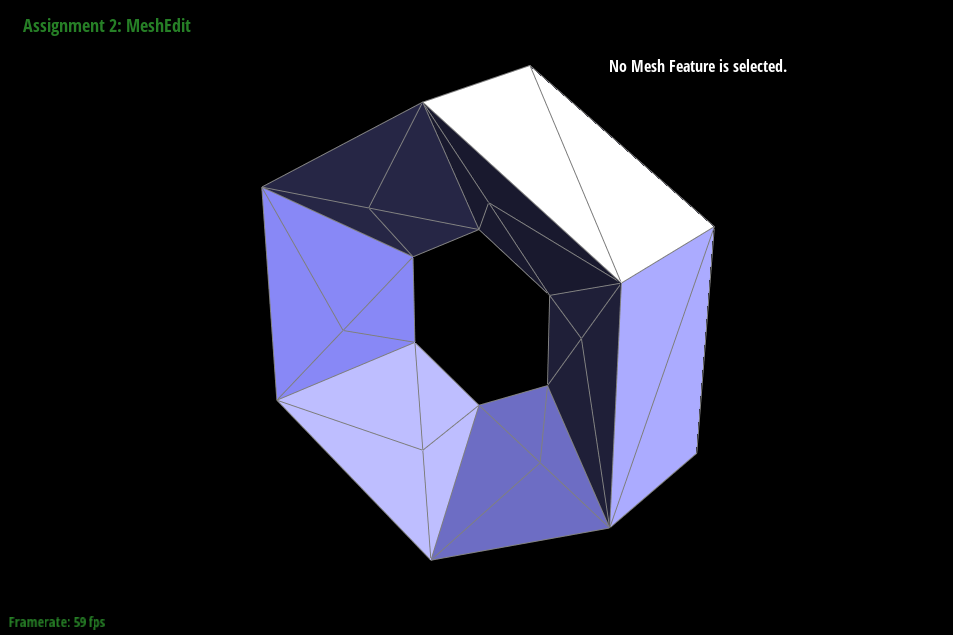
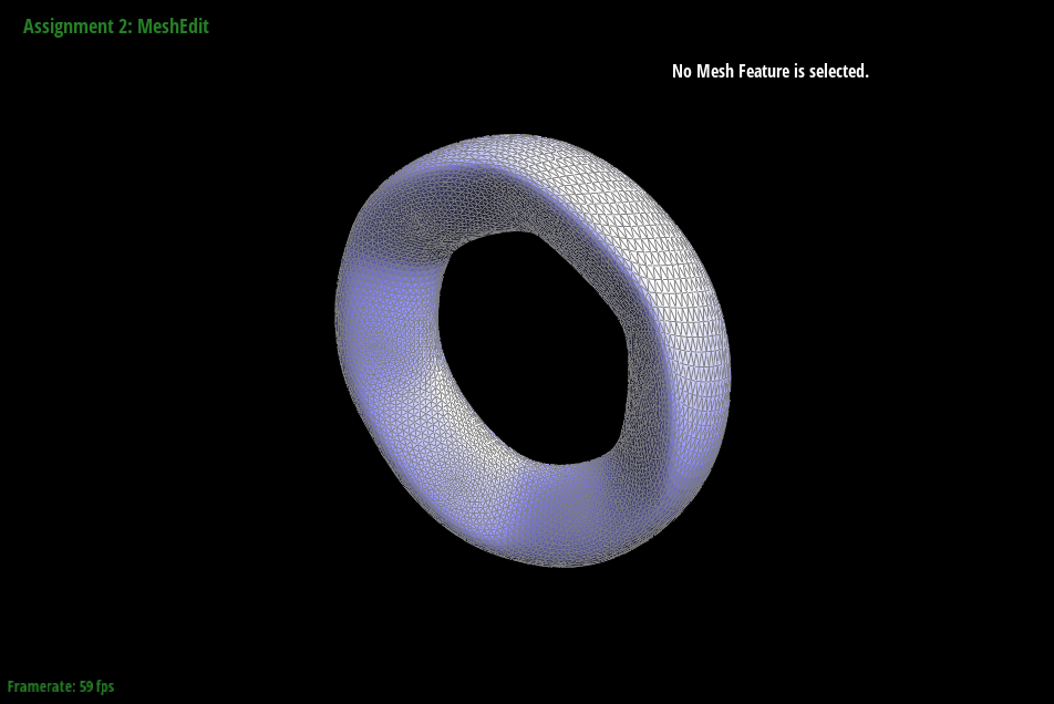
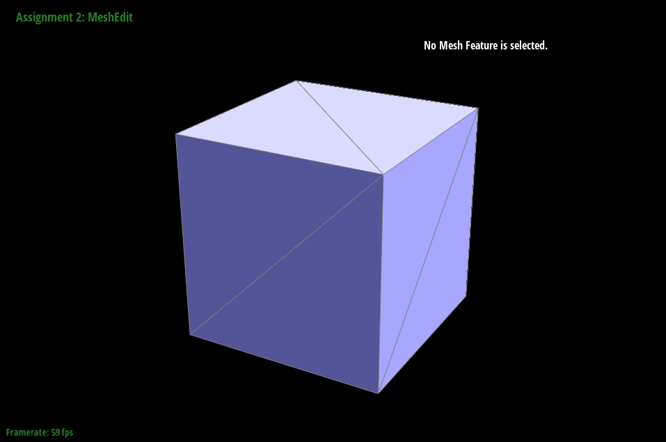
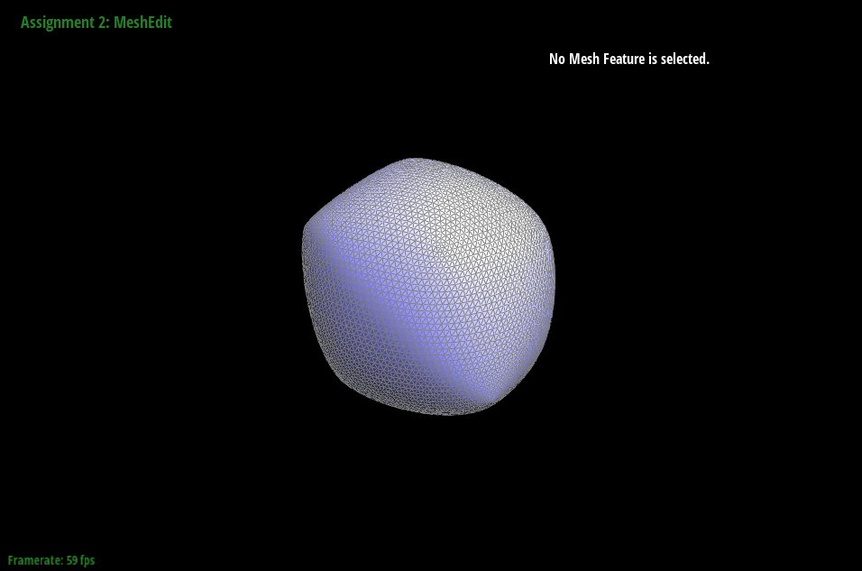
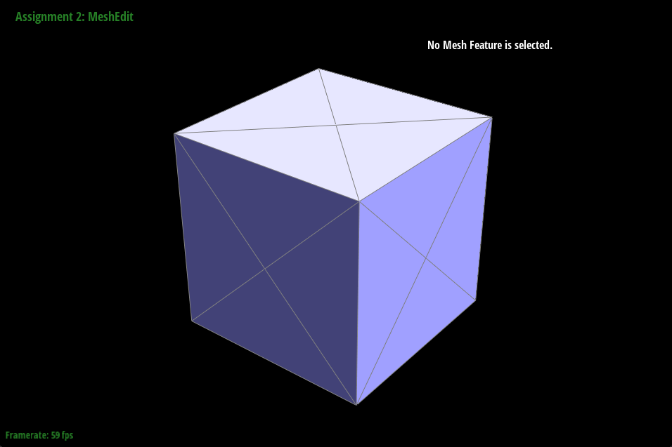
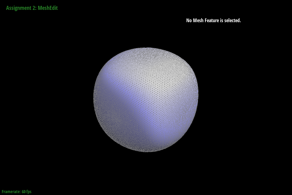
Below we document the results of Loop subdivision on a few of our meshes, and some interesting pre-processing techniques that we can do to manipulate the results that we get. In Figure 9, we can see that sharp corners and edges get smoothed out after performing Loop subdivision. In Figure 10, we can see that by pre-splitting some edges, we can reduce this smoothing effect that we see with Loop subdivision, where we can clearly see that the angularity of the outer ring is more pronounced than in Figure 9. In Figure 11, we can see that for the cube mesh, it becomes asymmetrical after a few levels of Loop subdivision. This is because not every vertex in the cube has the same degree. The vertices with degree 3 are less restrained by neighboring vertices when computing positional updates causing this asymmetry. This can fixed so that the cube subdivides symmetrically by splitting the edges on each face of the cube so that all of its vertices now have the same degree. We can see this effect below in Figure 12. In Figure 12, we can see that by pre-splitting the edges on the faces of the cube, we can make the cube subdivide symmetrically.