Overview

In this assignment, we reinforced many of the ideas derived from lecture, rendering images with various techniques; we started off with ray-scene intersection and implemented algorithms to accurately detect where rays intersect with objects in the scnee. Then, we implemented an acceleration/optimization for these intersection tests by organizing bounding volume hierachies, so that we could efficiently check for ray intersections. This optimization significantly reduced rendering times and allowed for us to render images that would have taken a really really long time. After, we explored how light reflects off of surfaces and implemented an estimator for the reflection equations in lecture to capture reflection characteristics of materials. In the end, we generated images using monte carlo path tracing and using direct and indirect illumination, we rendered a more realistic scene. To optimize this further, we introduced adaptive sampling, another optimization for solving our noise/speed tradeoff problem with sampling. In adaptive sampling, instead of having a fixed number of samples per pixel, we weighted the number of samples of pixel by how fast they would converge. Although the assignment was undoubtedly long and, in some parts, frustrating, we definitely believe it was worthwhile to be able to render these scenes and visualize how realistic and important lighting can be in a scene.

Part 1: Ray Generation and Scene Intersection (20 Points)

Walk through the ray generation and primitive intersection parts of the rendering pipeline.

For a given point, we generate ns_aa samples offset from the origin and scaled by the sampleBuffer dimensions (normalized coordinates). We then call generate_ray on our new sample points, which we implemented to convert the 2D coordinate into a 3D ray (by transforming the ray's direction vector to world space via camera 2 world matrix and scaled by hFov and vFov). We then evaluate the radiance of the newly sampled ray (finding the point of intersection from primitives and evaluating the radiance) and add to our uniformly weighted sum. In the last step, we update the pixel to this new average.

Explain the triangle intersection algorithm you implemented in your own words.

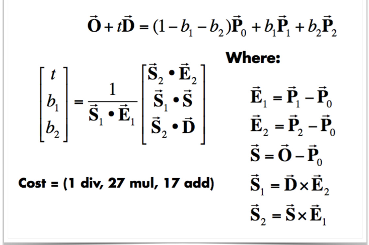
Our triangle intersection algorithm follows the optimized Moller Trumbore Algorithm from lecture (shown below), using barycentric coordinates. We derive barycentric coordinates of the intersection point, from the vectors derived from the calculations below. The parameter t represents the distance from the ray's origin to the intersection point, and we can use this point t to verify if it's within the bounds of the triangle (akin to the logic we had in assignment 1 of checking if a point is in a triangle).

Show images with normal shading for a few small .dae files.

Part 2: Bounding Volume Hierarchy (20 Points)

Walk through your BVH construction algorithm. Explain the heuristic you chose for picking the splitting point.

Our BVH construction algorithm relies on recursively creating children until we have size <= max_leaf_size (base case). We choose to split axis based on the surface area heuristic (selecting the minimum) and we split primitives based on average centroid; the primitives to <= avg centroid axis will belong to left child recursion and what's left will belong to the right children recursion. Once we reach the base case, we create a leaf node with all the primitives and this propels the algorithm back up. The surface area heuristic intuitively allows us a simple but effective cost model where by tightening the number of triangles in a given space.

Show images with normal shading for a few large .dae files that you can only render with BVH acceleration.

Compare rendering times on a few scenes with moderately complex geometries with and without BVH acceleration. Present your results in a one-paragraph analysis.

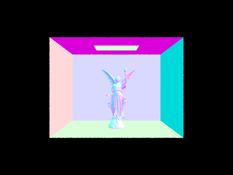
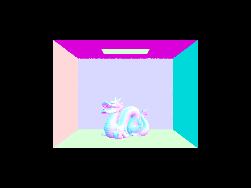
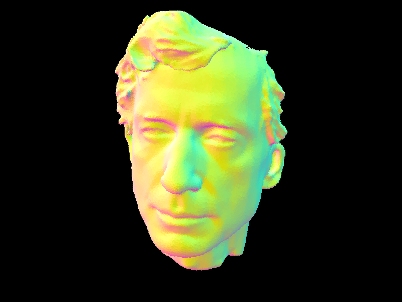
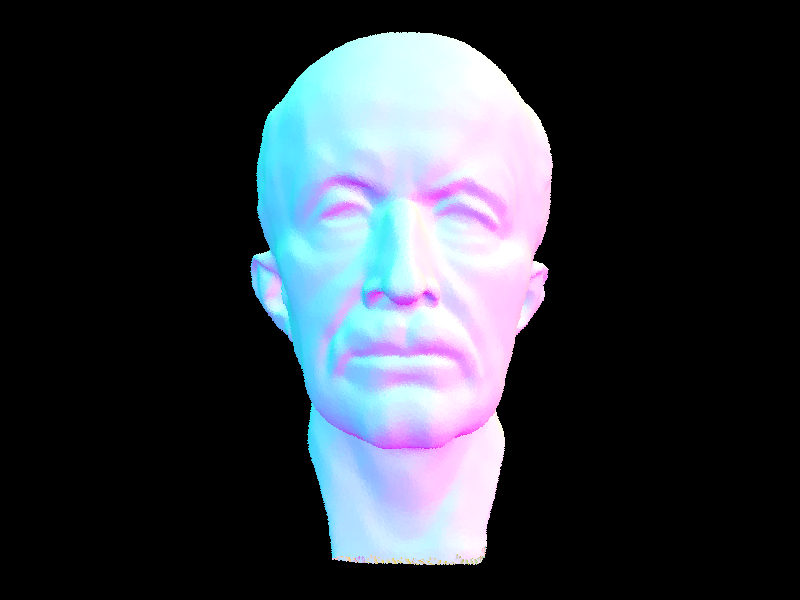
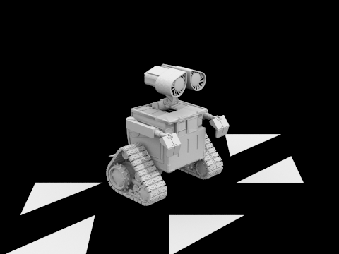
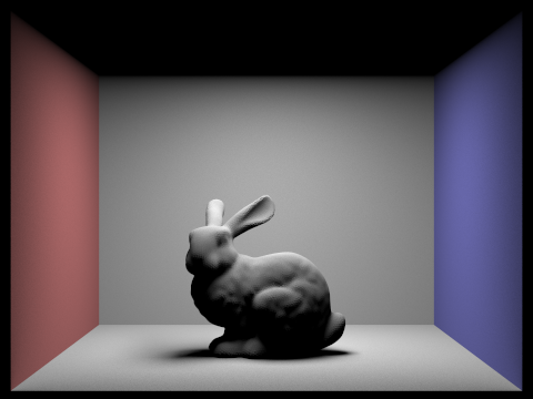
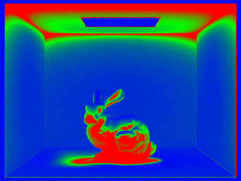
The rendering times without BVH acceleration for maxplanck.dae, beast.dae, peter.dae take 86.5, 149.5, and 75.8 seconds, respectively. Whereas, with BVH acceleration, they render almost instantaneously. Organizing the primitives into a tree structure allows for more efficient lookups of intersections, eliminating large portions of a scene that are not intersected by a given ray. This is confirmed through our testing as with BVH acceleration, the number of intersections tests (per ray) is around 2.5; whereas without BVH, the number of intersection tests (per ray) reaches thousands, depending on scene. The maintenance of this hierarchical structure allows us to test versus bounding volumes rather than the entire geometry of the primitives, which, as one can imagine, significantly reduces rendering time.

Part 3: Direct Illumination (20 Points)

Walk through both implementations of the direct lighting function.

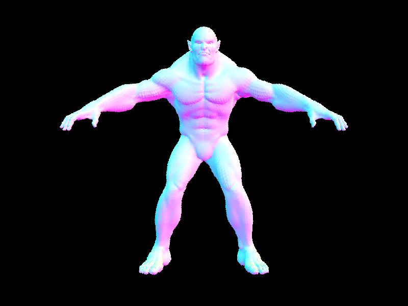
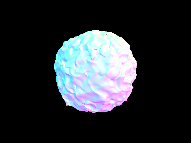
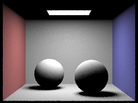
For hemisphere sampling, we uniformly sample from the hit point and generate a new ray based on this new direction (converted to world coordinates since Ray is in world space and the sample we generate is in object space). If the new ray intersects, we add the reflection sample (followed from reflection equation estimator in lecture). After we iterate through all the samples, we multiply by 1/pdf (weighted by pdf) and divide by num_samples to average. For importance sampling, we sample from each light source and for each light source, we sample a number of points on it (if the light source is a point light source we only need to sample once). We the ntest if the hitting point is the first object between itself and the light by testing if there's another intersection from the newly sampled ray (making sure the corresponding elements are correctly in space (world or object space). If there's no object blocking in between hit point and light source, then we sum using similar approach from hemisphere sasmpling. (task 3) Instead of having a uniform pdf, we have a pdf from the point on the light source.)

Show some images rendered with both implementations of the direct lighting function.

Focus on one particular scene with at least one area light and compare the noise levels in soft shadows when rendering with 1, 4, 16, and 64 light rays (the -l flag) and with 1 sample per pixel (the -s flag) using light sampling, not uniform hemisphere sampling.

Compare the results between uniform hemisphere sampling and lighting sampling in a one-paragraph analysis.

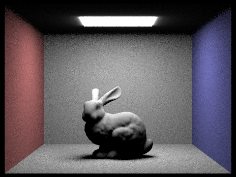
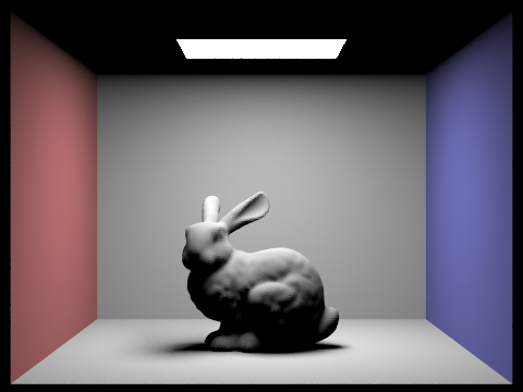
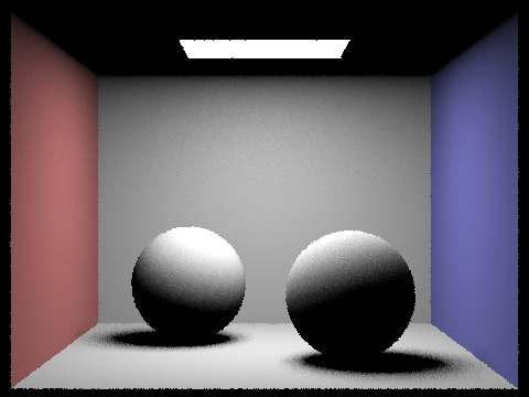
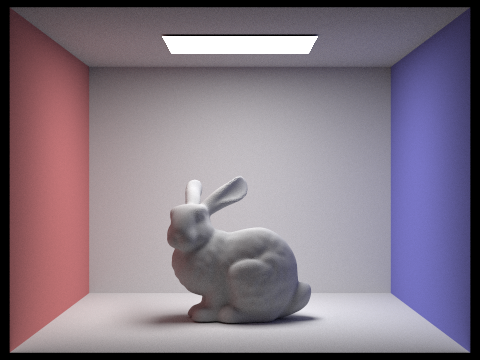
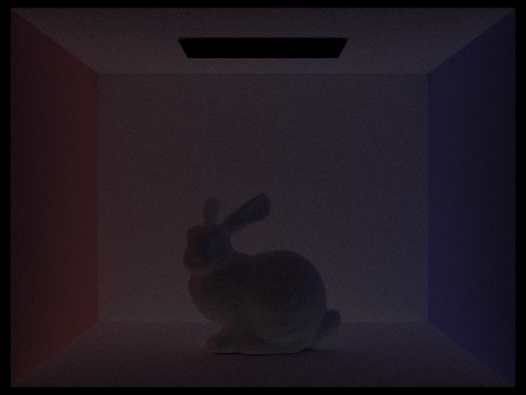
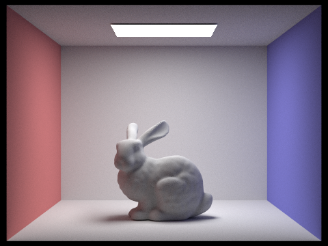
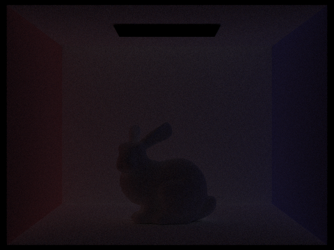
As seen above, the greater number of light rays we use, the better the image converges to its actual lighting. The difference in shadows between 1 light ray and 16 light rays per pixel is quite large. More notably, the backdrop of the scene seems to converge much faster than the actual object and shadows, at 16 light rays, the background seems to already be at its actual lighting, whereas even at 64 light rays, there seems to be a noticeable amount of noise on the object and shadows (the areas that are blocked). This may be due to the fact that in importance sampling, we consider a sample if there's nothing blocking it, but with shadows, if there's a large object between it and the light source, then it will converge relatively slower than if there wasn't anything in between.

Part 4: Global Illumination (20 Points)

Walk through your implementation of the indirect lighting function.

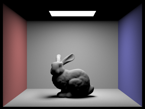
In this rendering process, the intuition is to recursively apply direct illumination, and we implemented an optimization to help terminate early via Russian roulette monte carlo. We basically implement the same illumination calculations from before (ensuring we're in the right object and world spaces for our calculations). Essentially, we explore many light paths from the source, but this can be costly so we introduce termination policies to optimize our algorithm. In russian roulette, we flip a coin that determines whether we terminate (this is weighted by probability of our choosing, in this case p=.4 probability of termination) and this solves our infinite recursion problem. If we don't terminate, then we follow similar procedure as before where we sample and estimate the reflectance equation we continue recursing until max_ray_depth is met. Our algorithm is also altered by presence of isAccumBounce variable, if this is false, then we only return the equation for the max_ray_depth bounce, instead of the total accumulated L_out.

Show some images rendered with global (direct and indirect) illumination. Use 1024 samples per pixel.

Pick one scene and compare rendered views first with only direct illumination, then only indirect illumination. Use 1024 samples per pixel. (You will have to edit PathTracer::at_least_one_bounce_radiance(...) in your code to generate these views.)

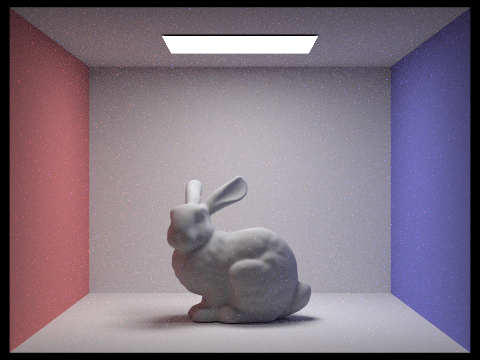
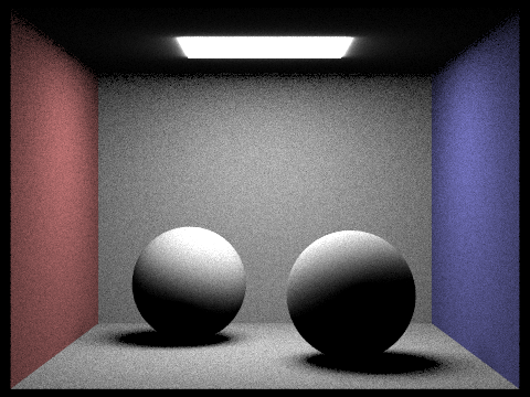
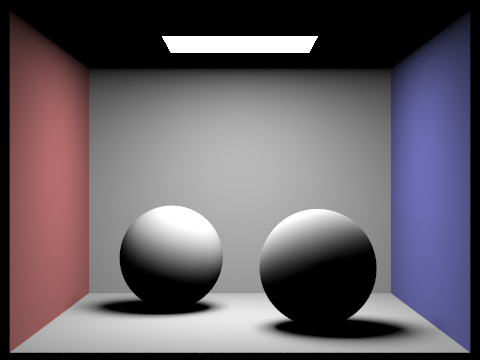
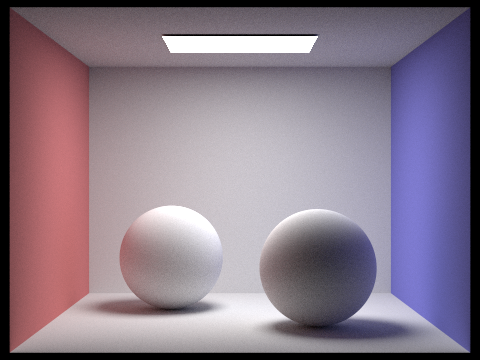
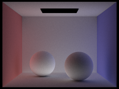
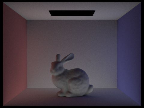
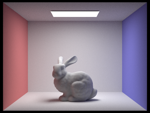
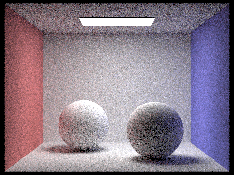
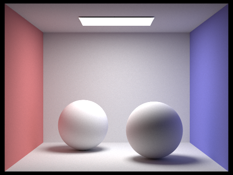
For direct illumination, we only use zero + one bounce lighting so we don't see the color reflect back onto the spheres from the walls. However, in indirect illumination, we see the presence of the color bleed effect onto the spheres since this is from the bounces after the first one bounce.

For CBbunny.dae, render the mth bounce of light with max_ray_depth set to 0, 1, 2, 3, 4, and 5 (the -m flag), and isAccumBounces=false. Explain in your writeup what you see for the 2nd and 3rd bounce of light, and how it contributes to the quality of the rendered image compared to rasterization. Use 1024 samples per pixel. (Left is isAccumBounces = False Right is isAccumBounces=True)

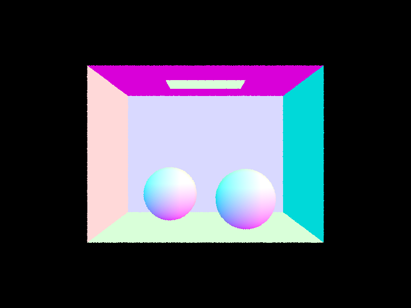
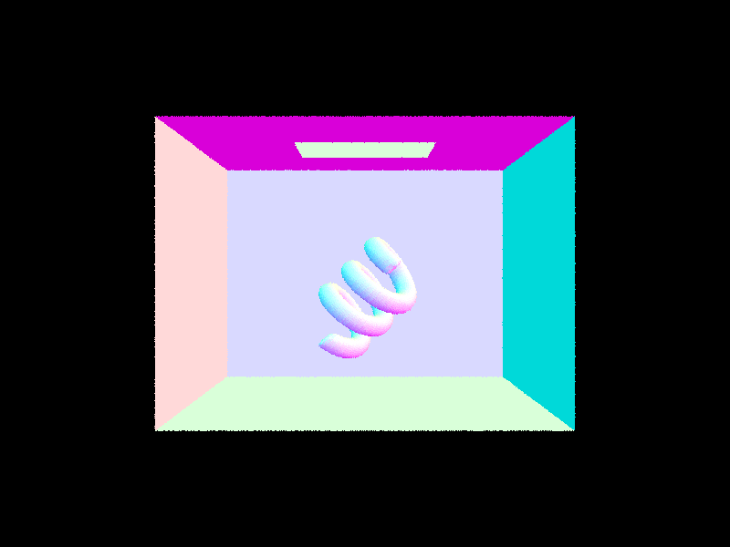
With the second and third light bounces, we see how they effect the environment since they've bounced off an object presumably. This results in more accurate and natural lighting as they introduce more nuanced shading and color bleeding, introducing an element of realism. In rasterization, we don't seem to achieve a nearly accurate effective of reflected light, so these may just be skipped entirely.

For CBbunny.dae, compare rendered views with max_ray_depth set to 0, 1, 2, 3, and 100 (the -m flag). Use 1024 samples per pixel.

There are drastic differences between m=0,1 and 2. 0 and 1 are basically direct illumination, and as we factor in rays beyond m=2 (indirect illumination), it begins to get difficult to tell the differences between further iterations. It's hard to spot any difference between m=100 and m=3

Pick one scene and compare rendered views with various sample-per-pixel rates, including at least 1, 2, 4, 8, 16, 64, and 1024. Use 4 light rays.

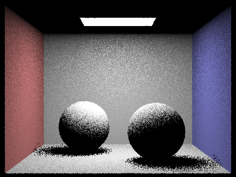
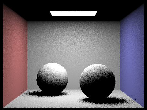
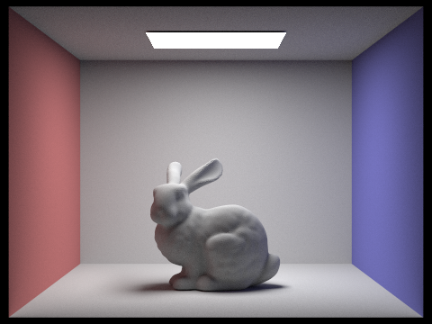
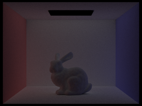
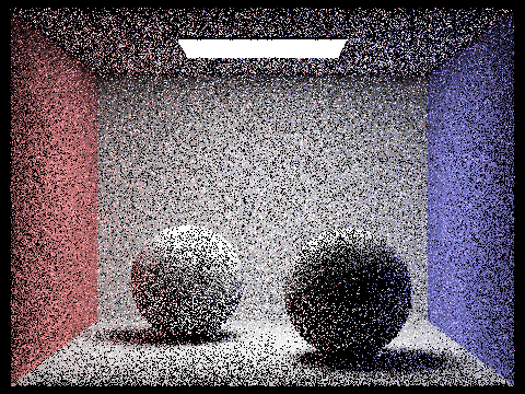
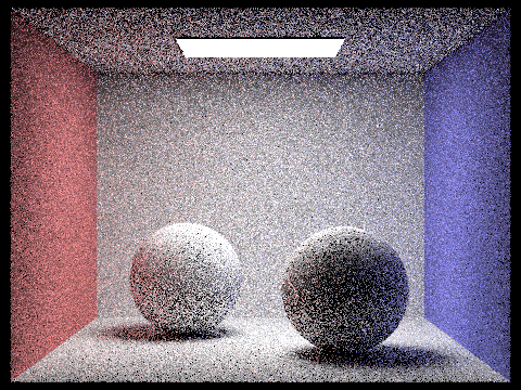
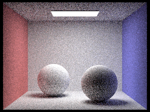
To summarize: while the effects from direct + indirect (global) illumination are great, we require a significantly large number of samples per pixel to reduce the noise. Even at 64 samples per pixel, we can see very apparent noise scattered through the scene. However, in 1024 samples per pixel, we can see a drastically more clear scene rendering. So, there's a clear tradeoff between rendering time and quality, as shown in the images above.

Part 5: Adaptive Sampling (20 Points)

Explain adaptive sampling. Walk through your implementation of the adaptive sampling.

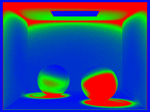
Without adaptive sampling, our monte carlo path tracing would have very visible noise when using a low amount of samples per pixel, so as a solution, we just increase the number of sample per pixel. However, we don't have to have the number of samples per pixel fixed for each pixel, we can use adaptive sampling to weight certain pixels more than others (depending on how fast they converge). In our adapative sampling algorithm, we check every ith iteration where i == samplesPerBatch for convergence. We compute the factor I by multpying 1.96 * std_deviation and dividing by the sqrt(total samples so far). The mean and variance is computed via s1/total samples_so_far where s1 is the running sum of illuminance. The variance is computed by (1/total_samples_so_far-1) *(s2-(s1^2)/totalsamples_so_far) where s2 is the running sum of the illuminance squared. If our factor I is <= maxTolerance * mean, then we terminate the sampling loop and update our sampling buffer.

Pick two scenes and render them with at least 2048 samples per pixel. Show a good sampling rate image with clearly visible differences in sampling rate over various regions and pixels. Include both your sample rate image, which shows your how your adaptive sampling changes depending on which part of the image you are rendering, and your noise-free rendered result. Use 1 sample per light and at least 5 for max ray depth.