lol i thought this pic was funny with the tiny cloth in the abyss

lol i thought this pic was funny with the tiny cloth in the abyss
The goal of this project is to build a cloth simulator using a mass and spring system. We implement everything from the actual creation of the cloth to its real-time movement to collisions with other objects. The cloth itself is made up of a mass and spring system, and we use numerical integration to simulate the actual movement of the cloth. From there we could move further into creating a realistic cloth simulator by handling collisions, with a sphere, a plane, and itself. The self collisions allow for the cloth to realistically fall and fold onto itself, while the sphere collision allows us the view the cloth and its properties as it is draped over something. The sphere collision proved extremely helpful in the last part of this project, which was creating shaders to model different textures on the cloth. We created these shaders using the language GLSL, and we used Blinn-Phong shading to create a more realistic look for the cloth. We also added additional shaders to add even more detail to the cloth, such as bump and displacement shaders, which add a 3D texture to the otherwise flat cloth.
Overall, it was extremely cool to see the final product of the cloth simulation, and how realistic it looks especially after we add the different shaders. We ran into quite a few difficulties implementing the physics of the cloth itself, such as with the movement simulation and the self-collisions, but it was very fascinating to see how it all came together in the end.
Take some screenshots of scene/pinned2.json from a viewing angle where you can clearly see the cloth wireframe to show the structure of your point masses and springs.
The goal of this section was to create a grid of masses and springs. First, we iterated through num_height_points and num_width_points via an inner loop to generate the point masses in row-major order, alongside the masses being evenly spaced. Based on the orientation (horizontal or vertical), we varied across the xy plane or the xz plane. If the point mass's (x, y) index is within the cloth's pinned vector, we set the point mass's pinned boolean to true. The pinned boolean indicates whether the point mass will remain stationary/pinned throughout the simulation.
After creating the grid of point masses, we needed to create springs to apply the structural, shear, and bending constraints between point masses. These are the restraints indicating what constraints would be applied:
Below are images of the entire grid zoomed out and zoomed in when running ./clothsim -f ../scene/pinned2.json with initial configurations of ks = 5,000:
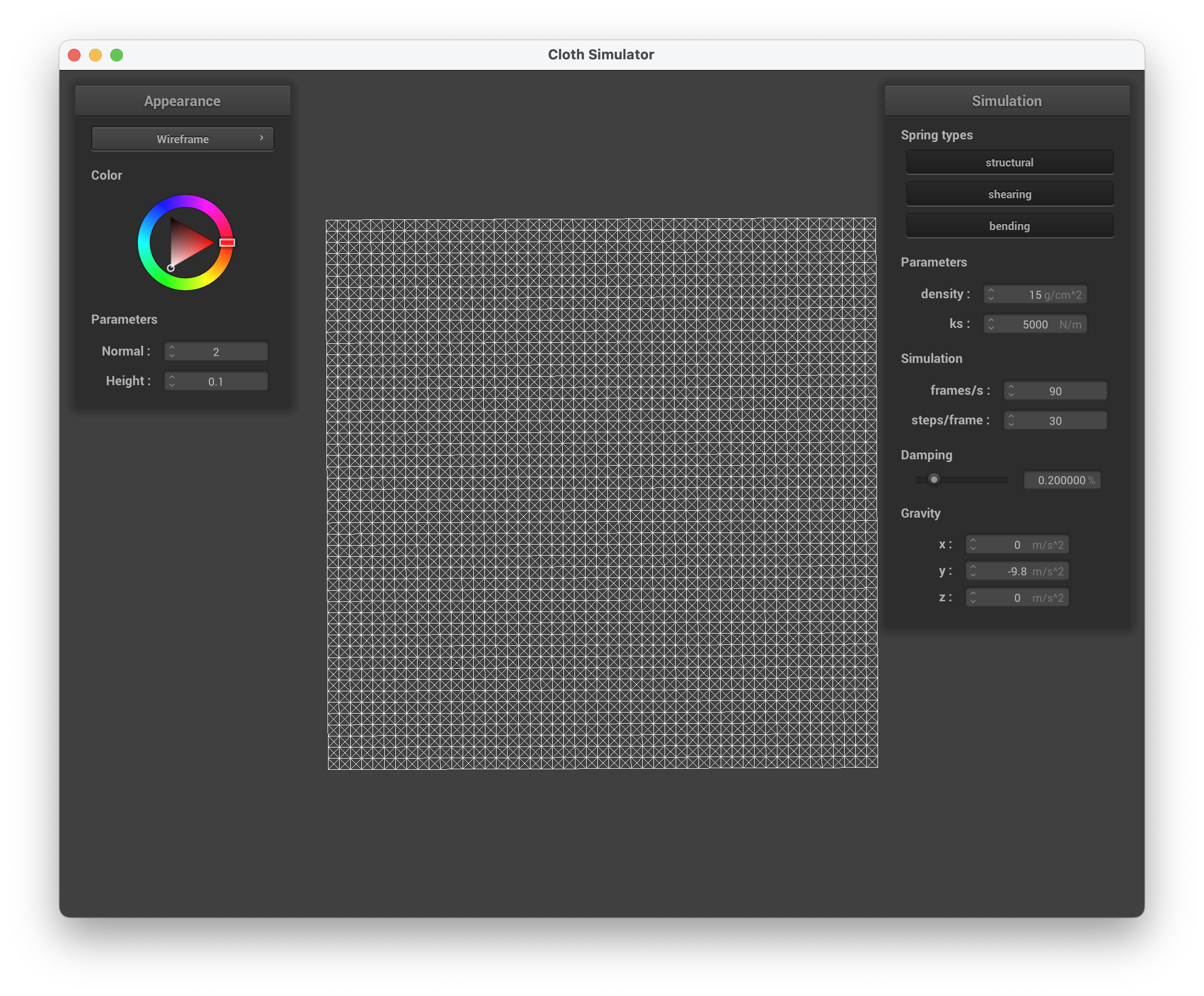
../scene/pinned2.json, entire grid
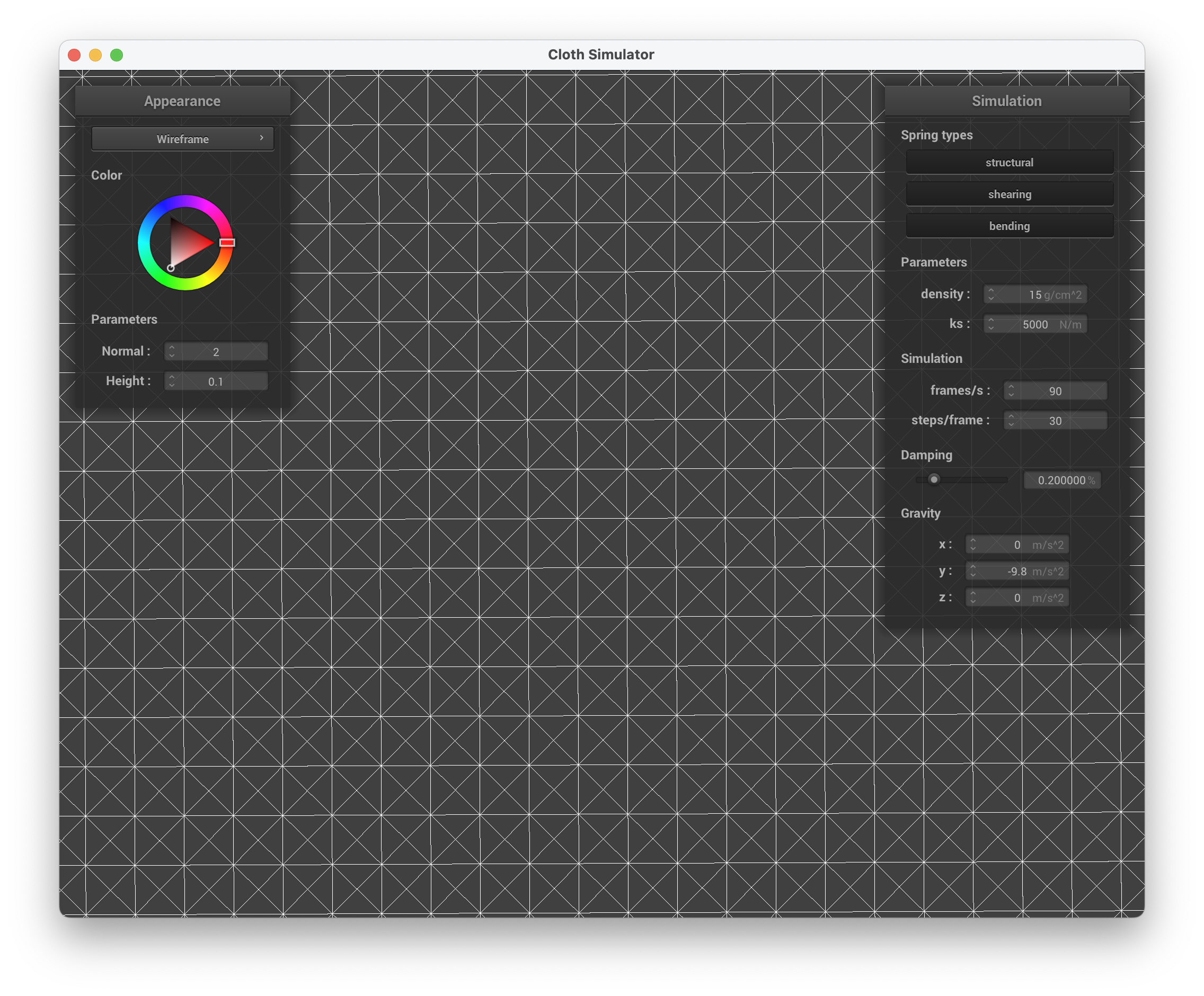
../scene/pinned2.json, entire grid zoomed
Below, we can see images of the grid with the different constraints applied:
Show us what the wireframe looks like (1) without any shearing constraints, (2) with only shearing constraints, and (3) with all constraints.
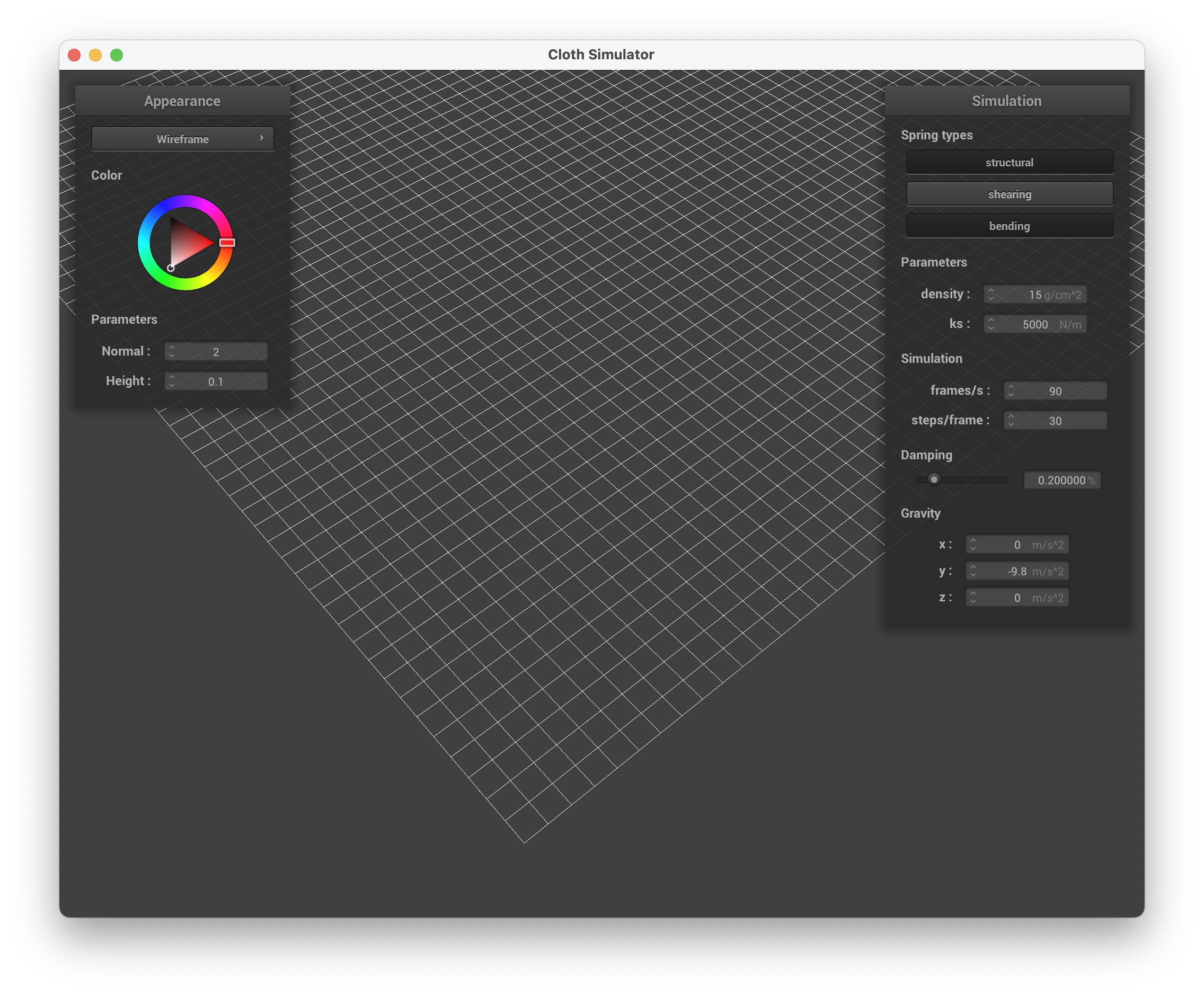
../scene/pinned2.json, without shearing constraints
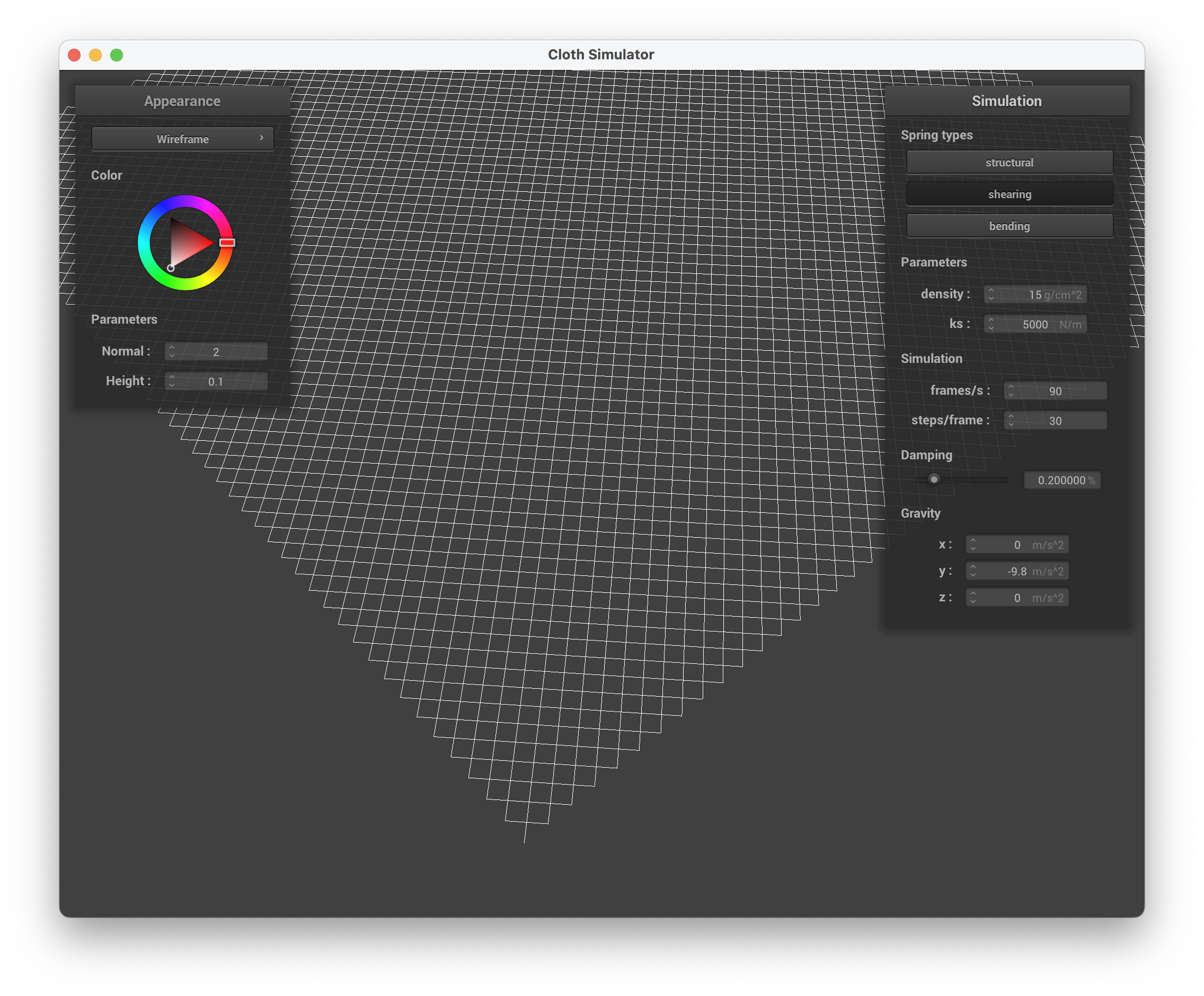
../scene/pinned2.json, with only shearing constraints
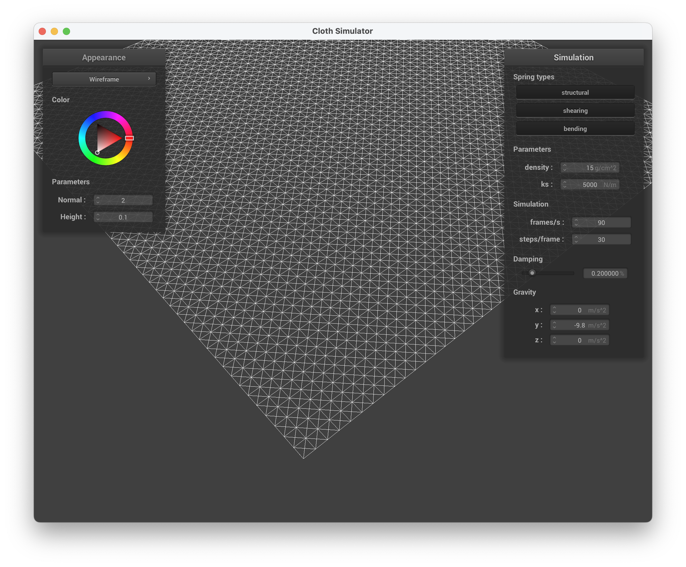
../scene/pinned2.json, with all constraints
In this task, we first calculated the external forces done by looping through the external_accelerations. All accelerations are applied uniformly so we summed all of the external_forces (a Vector3D) using Newton's 2nd Law (\(F = ma\)). Afterwards, we looped through all of the point masses and set each forces to external_force.
Next, we needed to apply the spring correction forces using Hooke's Law, \(F_s = k_s * (||p_a - p_b|| - l)\). For each spring, we apply \(F_s\) force to the point mass on one end and then an equal, but negated force on the other end. Bending constraints should be weaker than the other two constraints which is why we multiplied \(k_s * 0.2\).
In this task, we compute a point mass's new position by using Verlet integration on all unpinned point masses. The new position is calculated by \(x_{t+dt} = x_t + (1 - d) * (x_t - x_{t-dt}) + a_t * dt^2\). We also needed to update the point mass's last_position to the previous position prior to using Verlet integration.
Experiment with some the parameters in the simulation. To do so, pause the simulation at the start with P, modify the values of interest, and then resume by pressing P again. You can also restart the simulation at any time from the cloth's starting position by pressing R.
Describe the effects of changing the spring constantks; how does the cloth behave from start to rest with a very lowks? A highks?
To help keep springs from being unreasonably deformed during each time step, we implemented an additional feature based on the SIGGRAPH 1995 Provot paper on deformation constraints in mass-spring models. For each spring, we applied this constraint to prevent springs from extending more than 10% greater than its rest_length at the end of any time step.
If the spring's length doesn't extend more than 10% greater than its rest_length, we perform the following conditions to the point masses:
Below are images of running ./clothsim -f ../scene/pinned2.json with the default parameters of ks = 5000 N/m, density = 15 g/cm^2, damping = 0.2% to help showcase how experimenting with parameters causes the cloth to change.
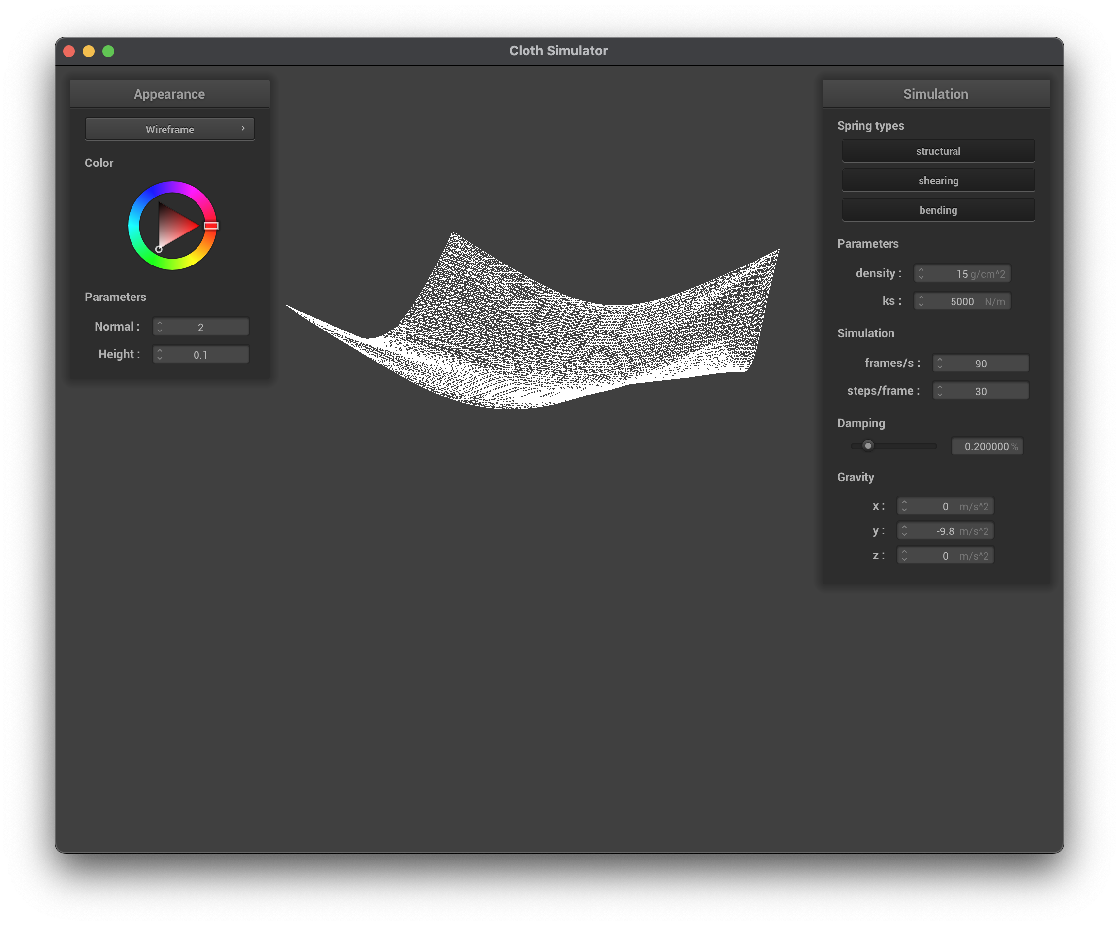
../scene/pinned4.json, final resting state, wireframe
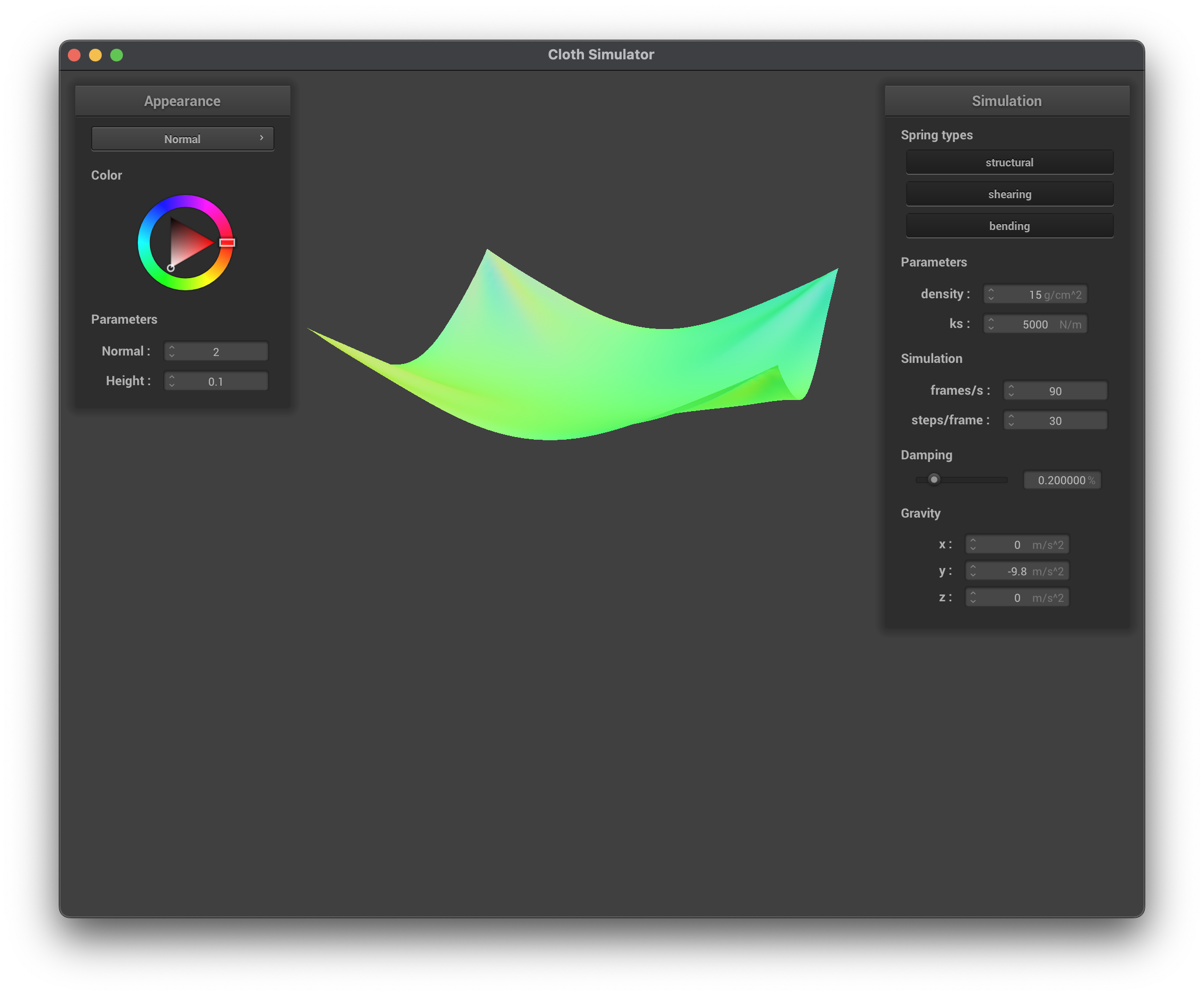
../scene/pinned4.json, final resting state, normal
For each of the below observe any noticeable differences in the cloth compared to the default parameters and show us some screenshots of those interesting differences and describe when they occur.
ks
When maintaining the default parameters (density, damping) and only modifying the spring constant, ks, we can see that as ks increases, the cloth becomes less malleable. This is because increasing the spring constant results in increasing the spring's stiffness, causing the cloth to appear less "creased" and more rigid/flat. At lower ks values, the strength of the springs is lower, hence why the cloth is more flexible and has more folds/creases.
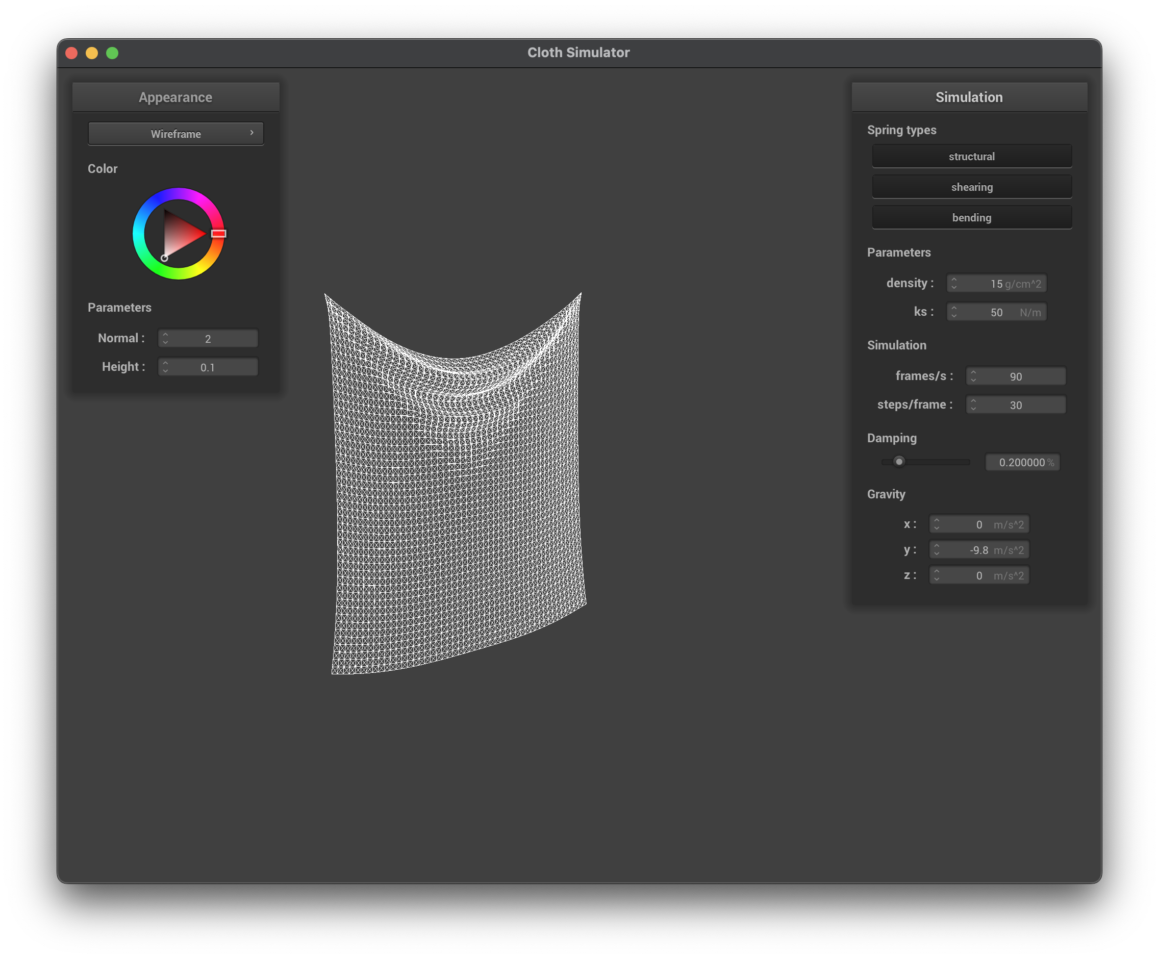
../scene/pinned2.json, ks = 50 N/m, wireframe
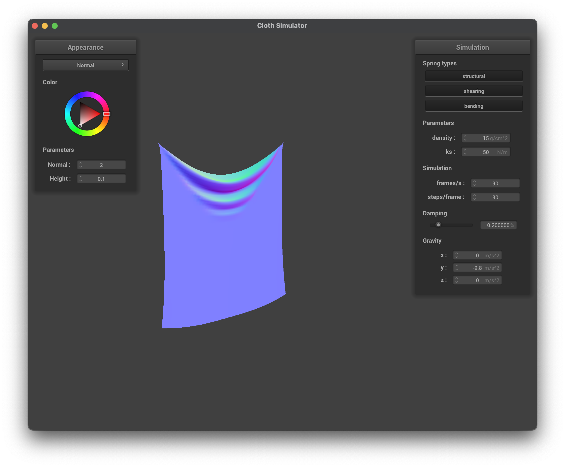
../scene/pinned2.json, ks = 50 N/m, normal
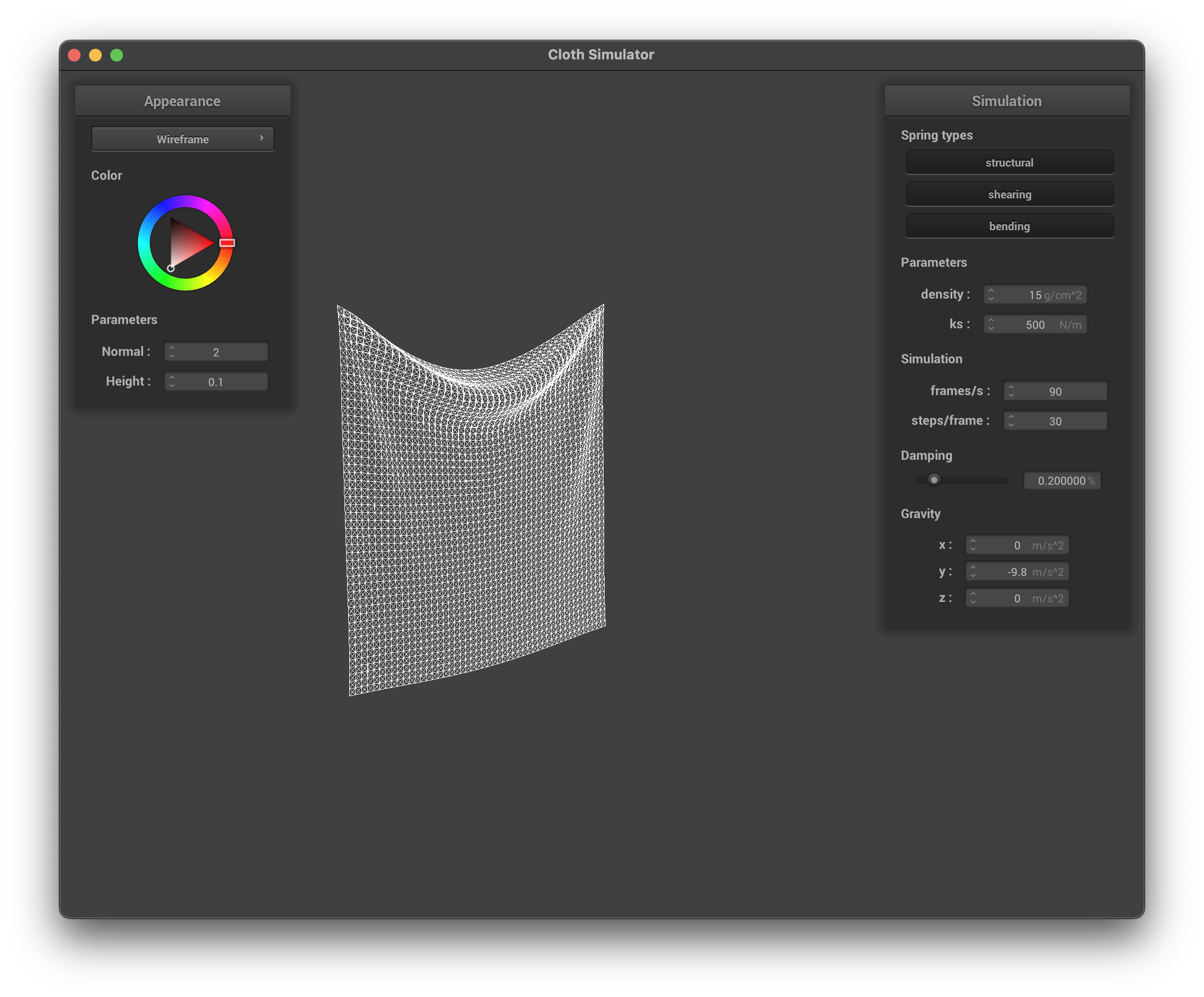
../scene/pinned2.json, ks = 500 N/m, wireframe
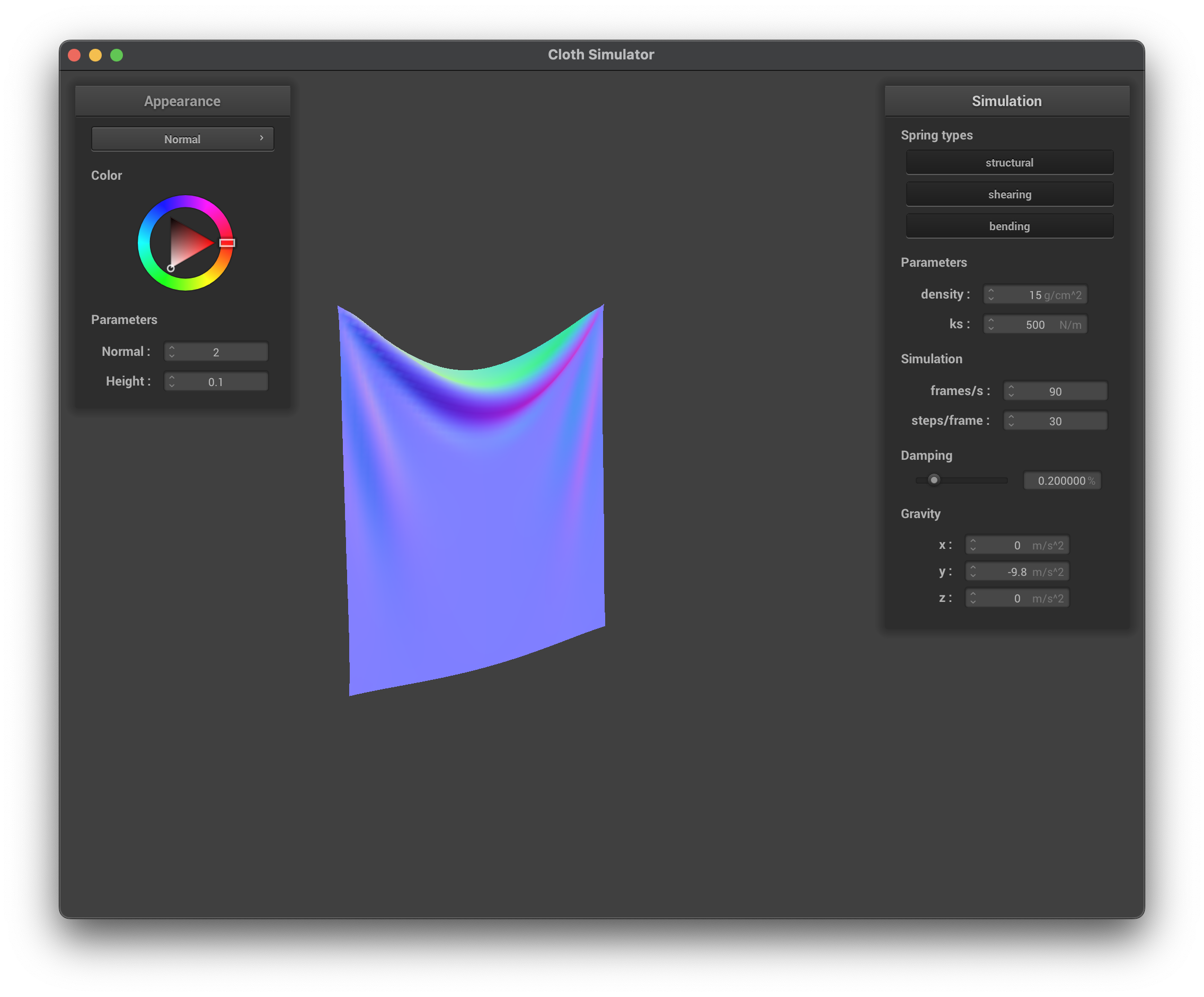
../scene/pinned2.json, ks = 500 N/m, normal
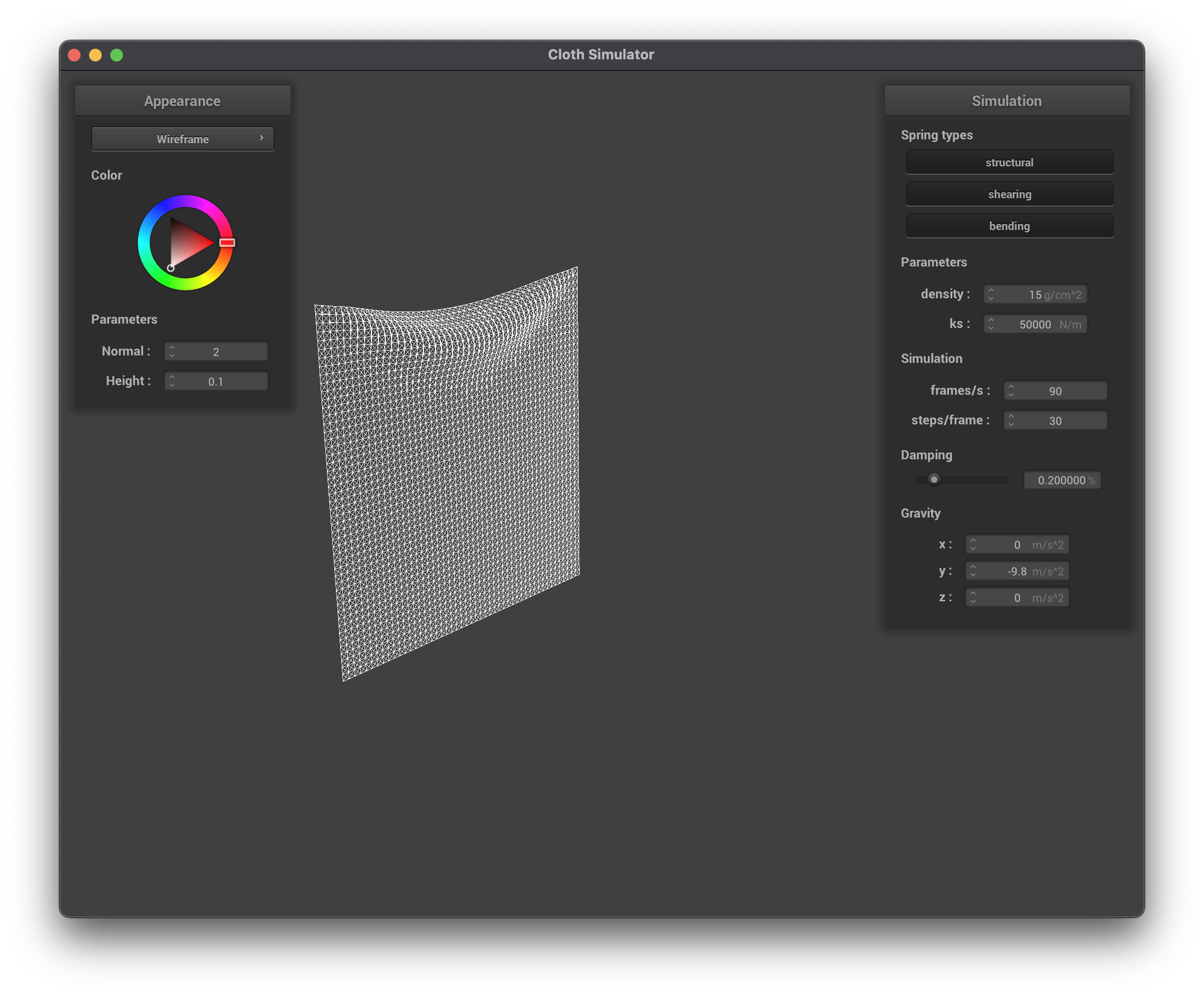
../scene/pinned2.json, ks = 50,000 N/m, wireframe
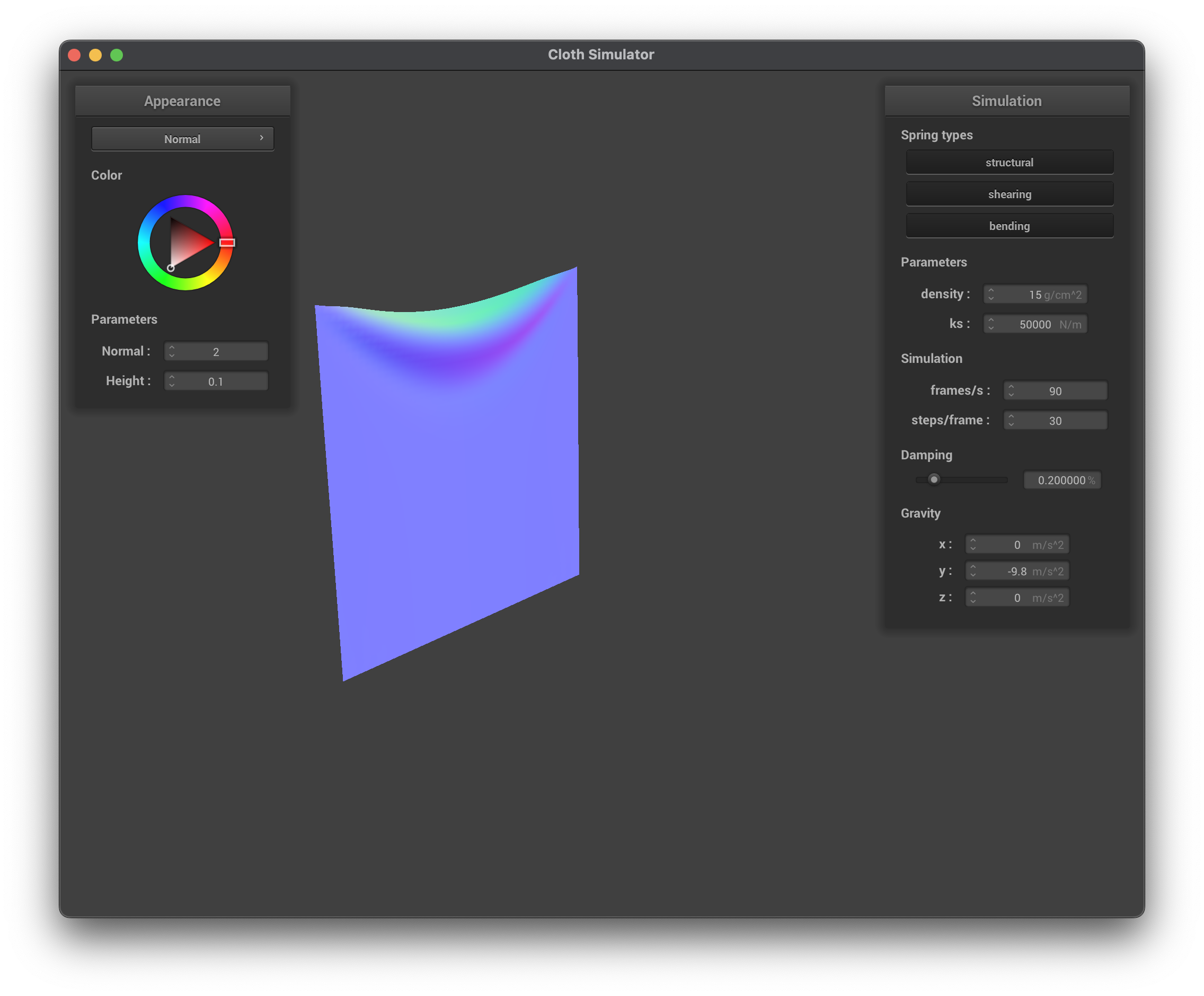
../scene/pinned2.json, ks = 50,000 N/m, normal
density
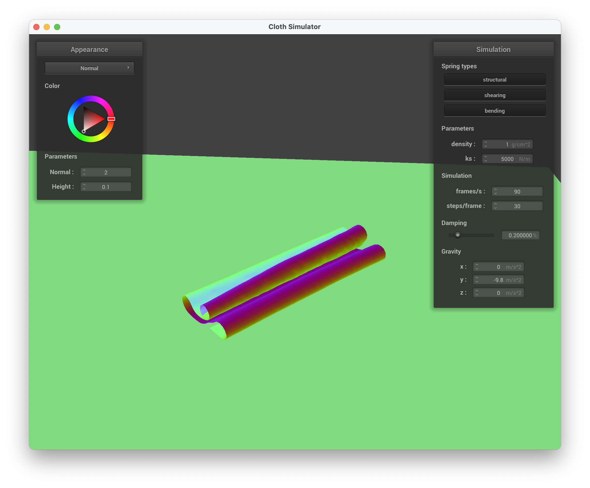
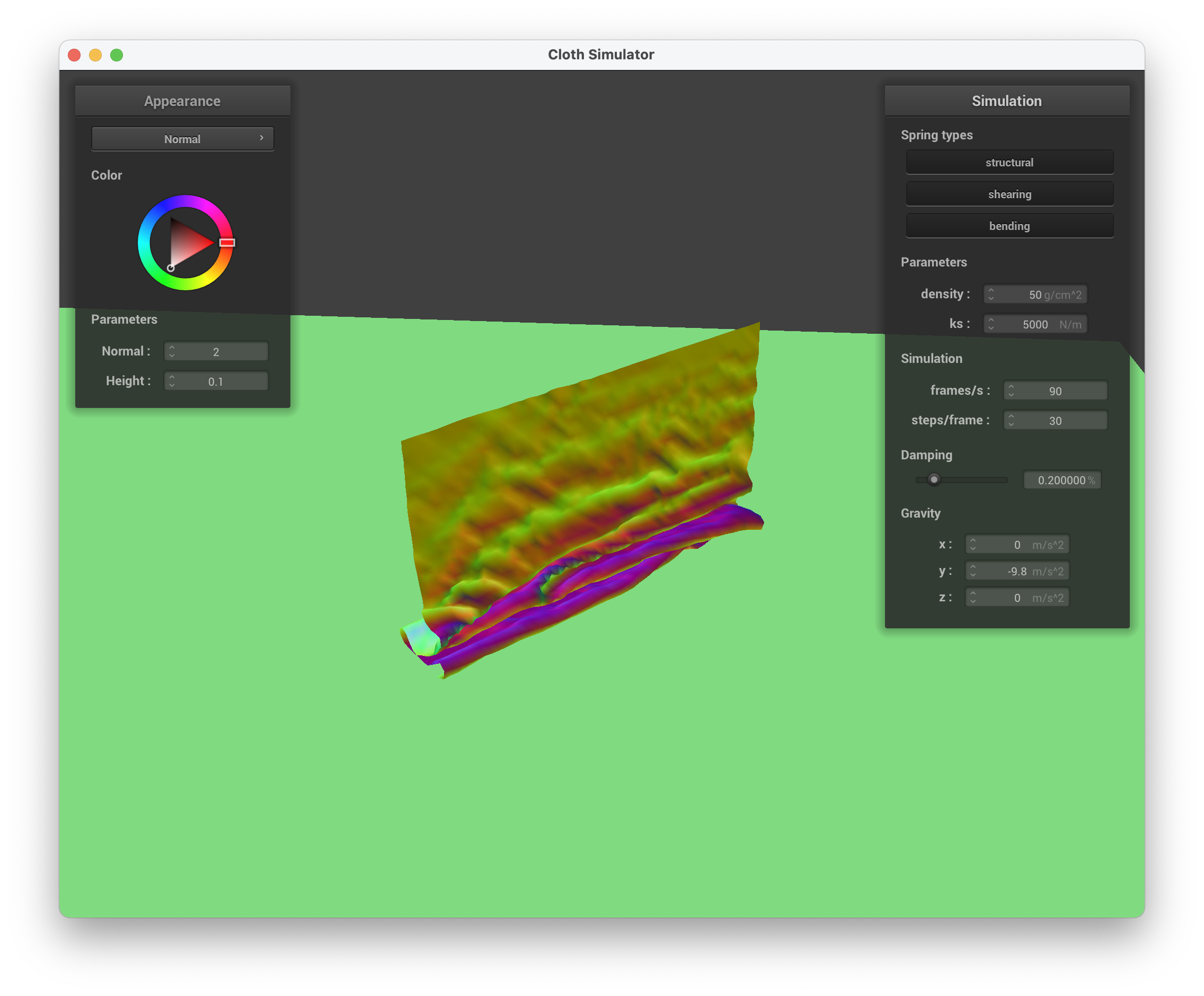
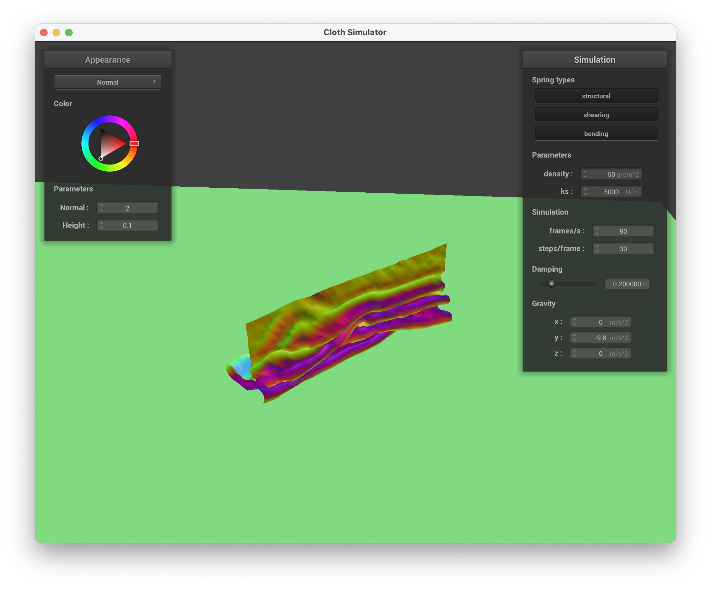
When maintaining the default parameters (ks, damping) and only modifying the density, we can see that its effect on the cloth is almost inversely to ks — increasing the density has similar results to the cloth as decreasing the ks. At lower density values, the cloth has lower mass. Using Newton's Second Law (\(F = ma\)), this means that the forces accumulated at each point mass will be less, causing less forces to pull the cloth down and ultimately resulting in less creases/folds in the cloth (more flat). At higher density values, the forces accumulated at each point mass are greater which is why there are more creases/folds in the cloth.
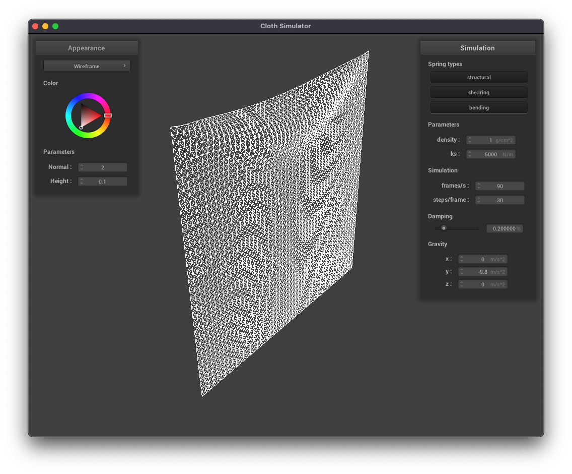
../scene/pinned2.json, density = 1 g/cm^2, wireframe
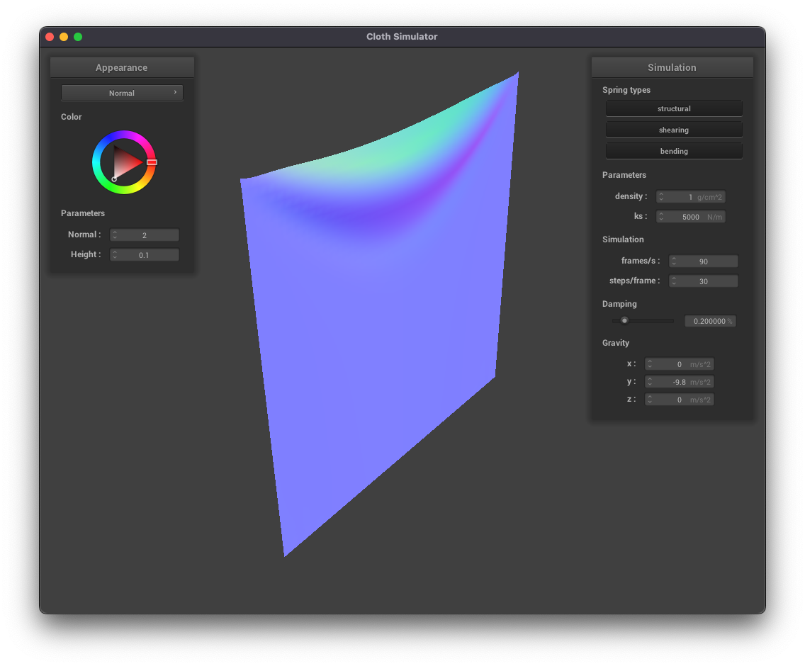
../scene/pinned2.json, density = 1 g/cm^2, normal
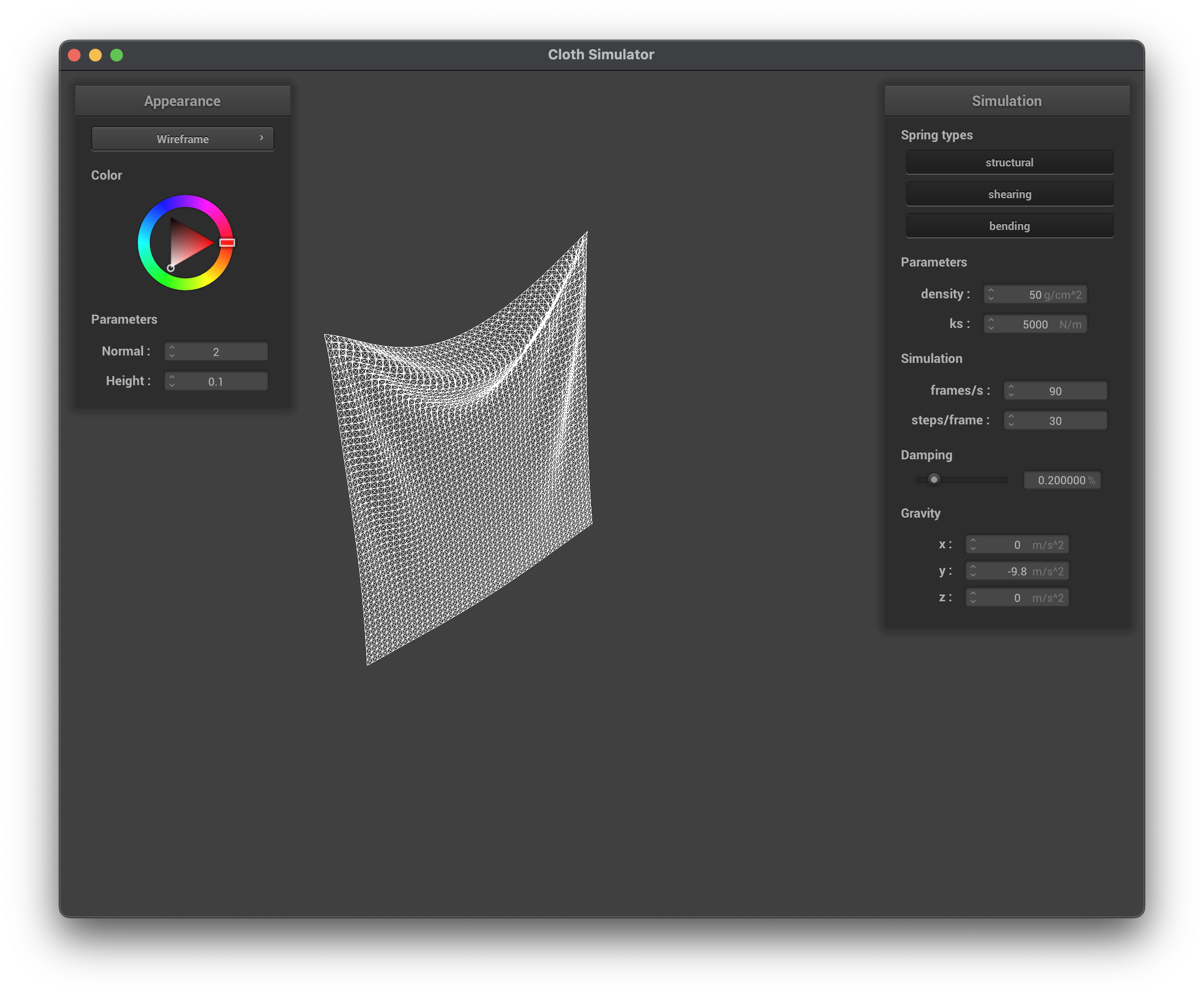
../scene/pinned2.json, density = 50 g/cm^2, wireframe
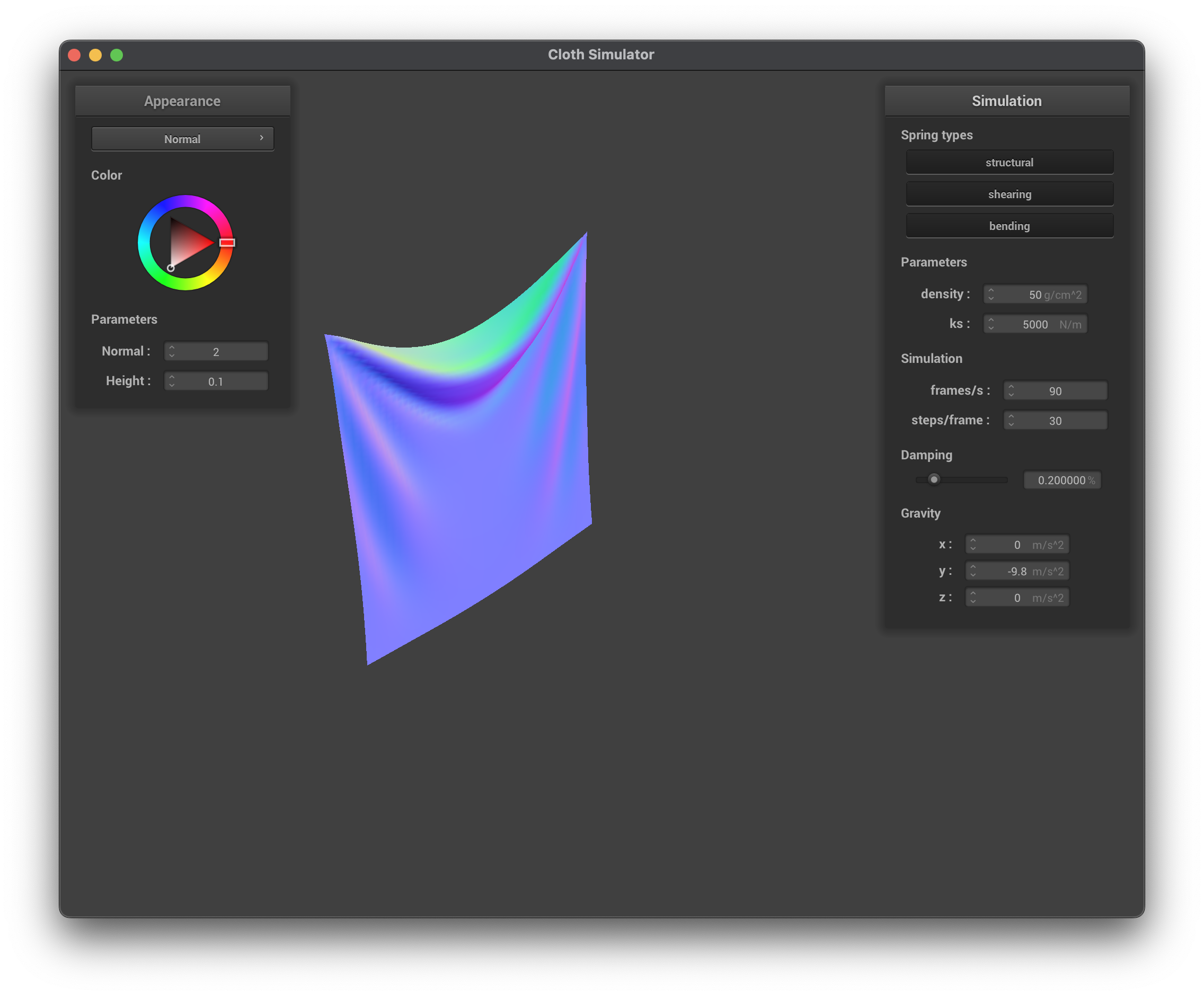
../scene/pinned2.json, density = 50 g/cm^2, normal
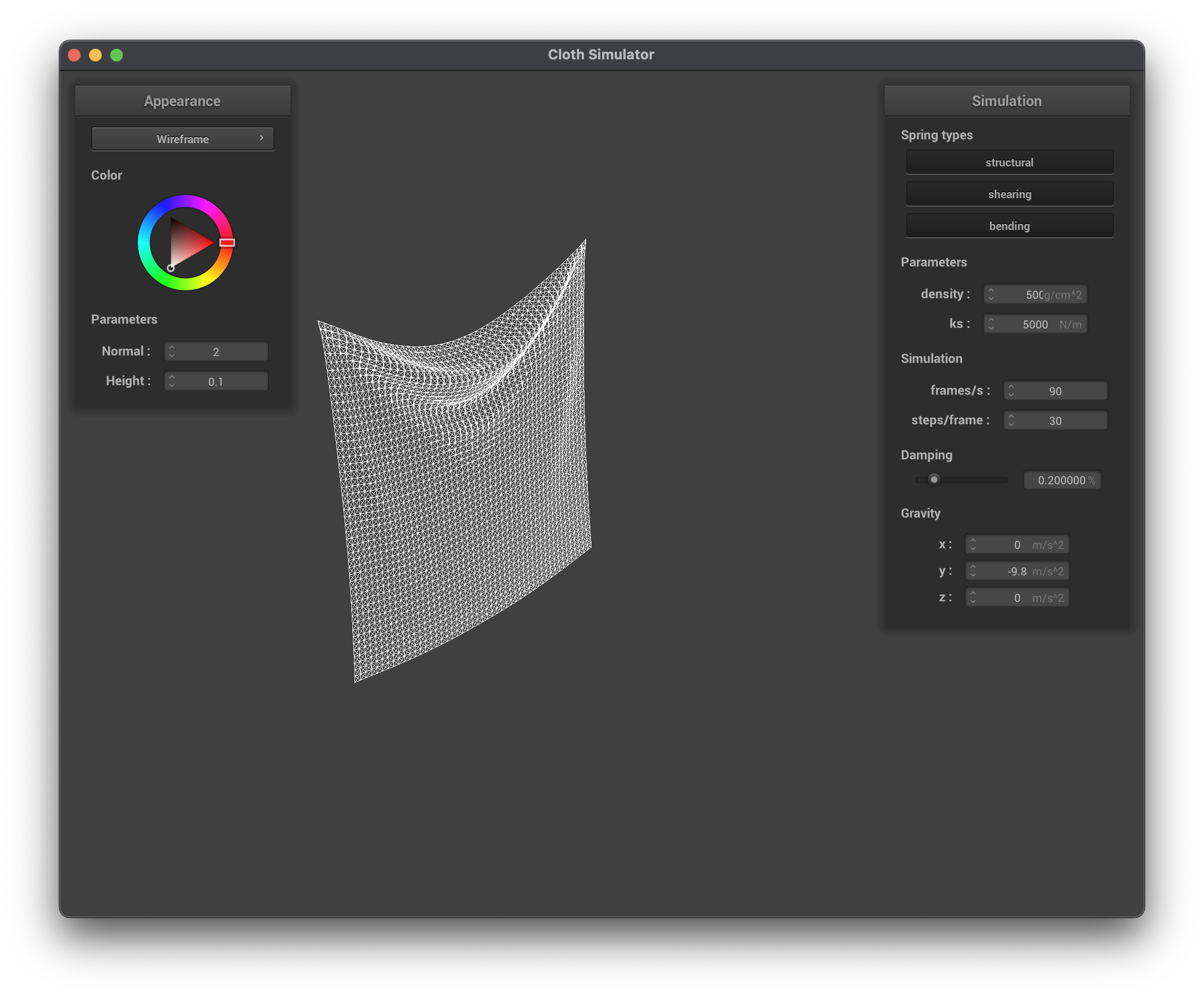
../scene/pinned2.json, density = 500 g/cm^2, wireframe
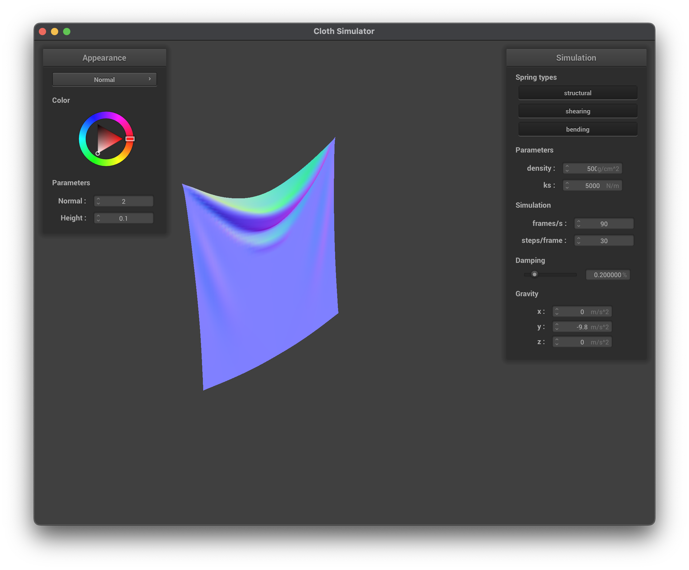
../scene/pinned2.json, density = 500 g/cm^2, normal
damping
When maintaining the default parameters (ks, density) and only modifying damping, we can immediately see that modifying damping impacts the speed at which the simulation/cloth reaches a state of rest. When damping is increased, this causes the cloth to stop its motion at a faster speed compared to a lower damping value. A higher damping causes the cloth to swing back and forth more rapidly. damping impacts the velocity value in Verlet integration so when damping is a lower value, there is no loss of energy, hence why the cloth rapidly swings. When damping is increased, the forces acting on the cloth are "dampened" and there is a loss of energy, hence why the cloth swings less rapidly. This is most evidently seen when comparing damping = 1 g/cm^2 and damping = 50000 g/cm^2.
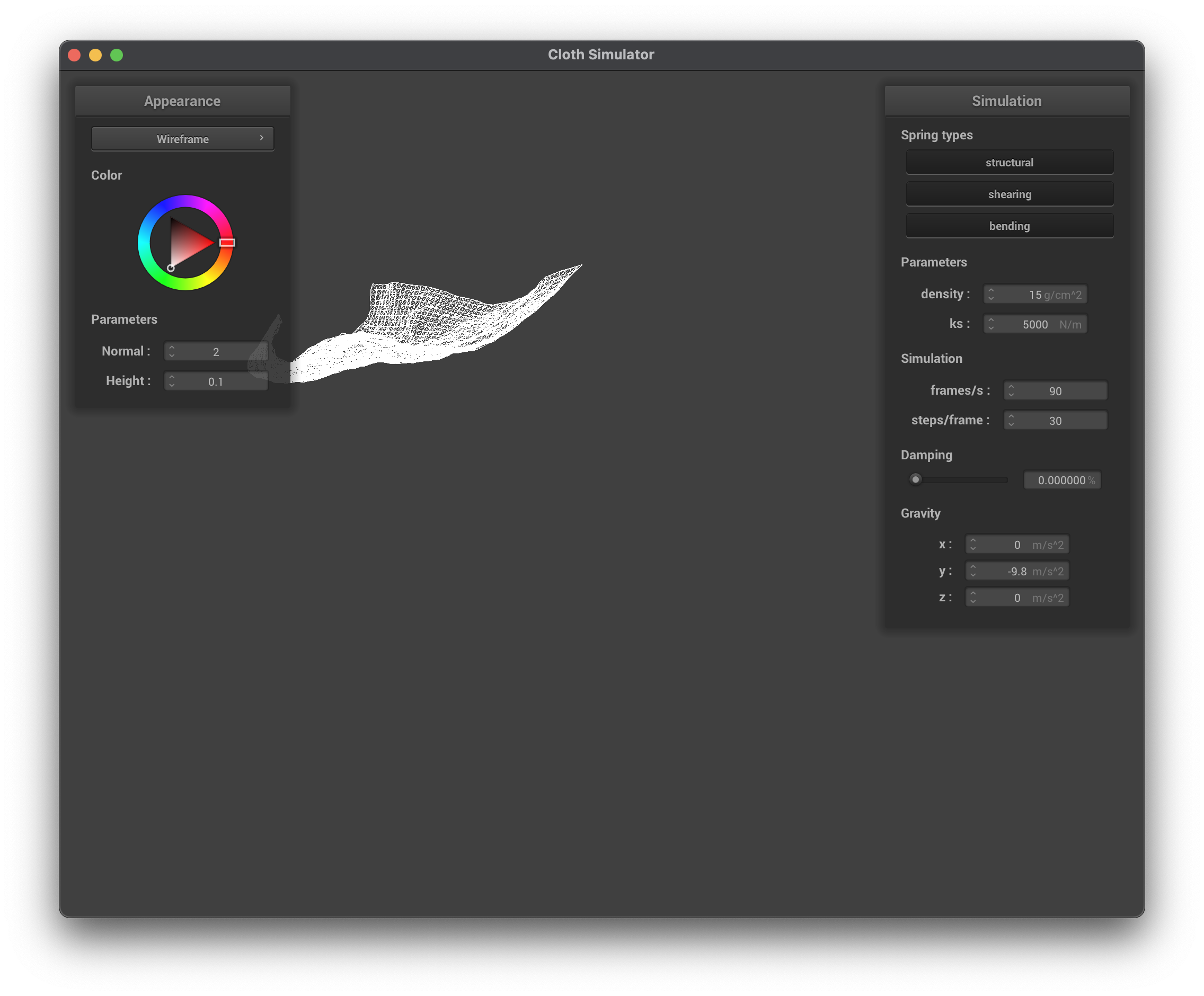
../scene/pinned2.json, damping = 0%, wireframe
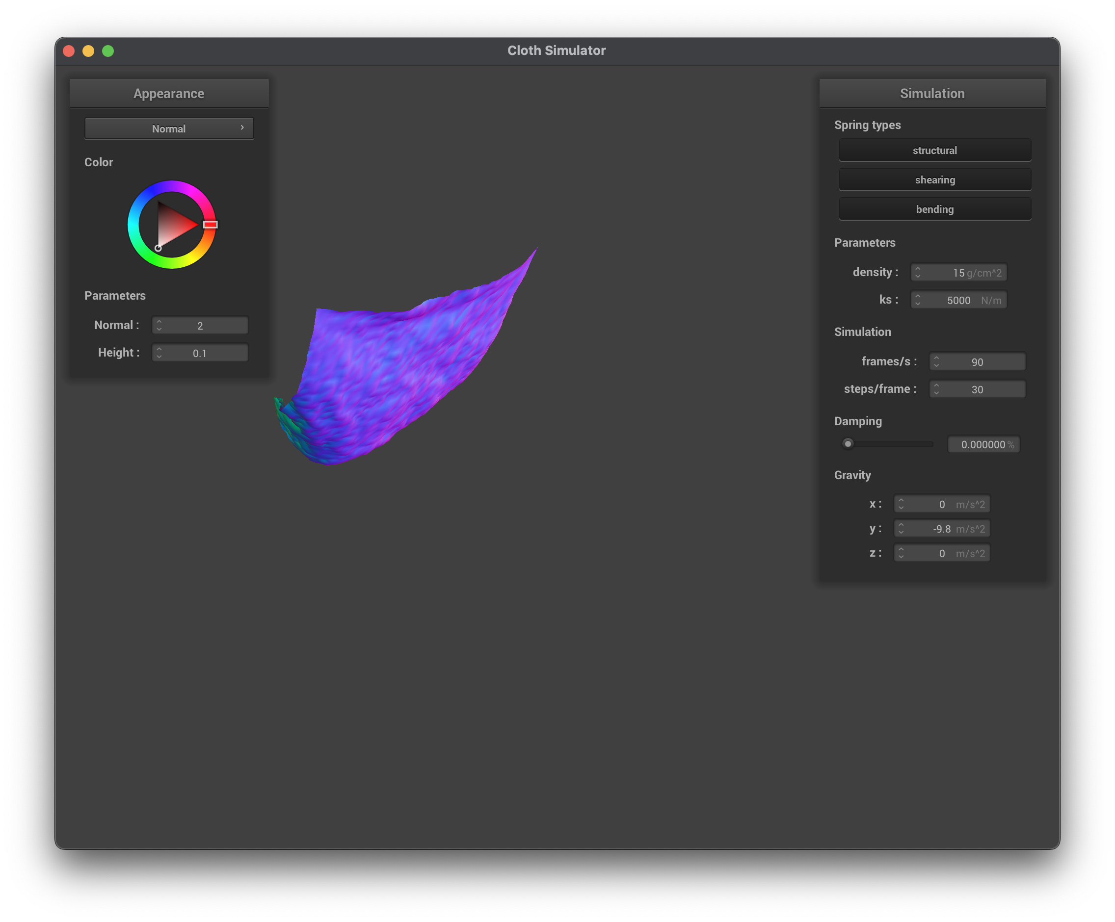
../scene/pinned2.json, damping = 0%, normal
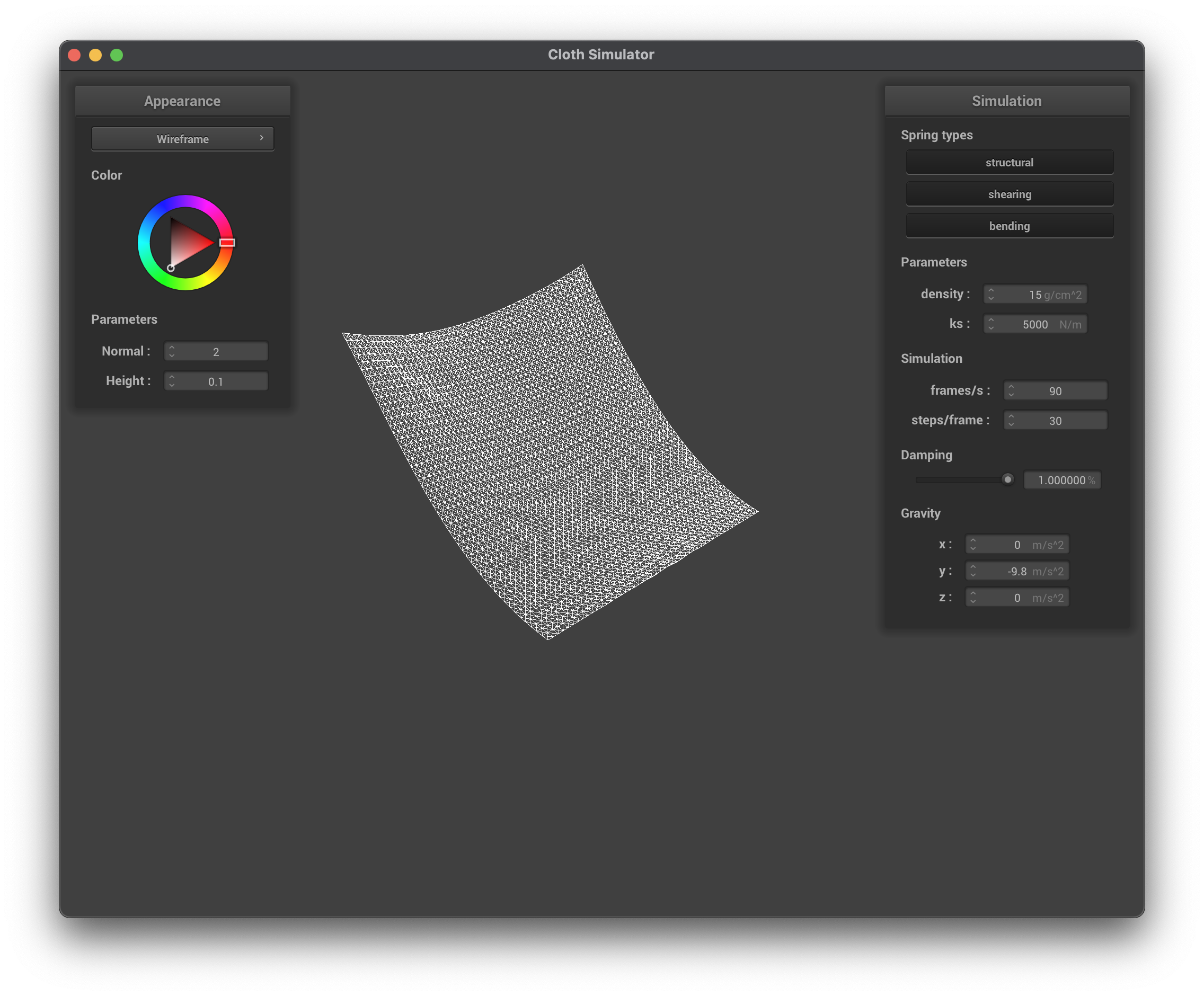
../scene/pinned2.json, damping = 1%, wireframe
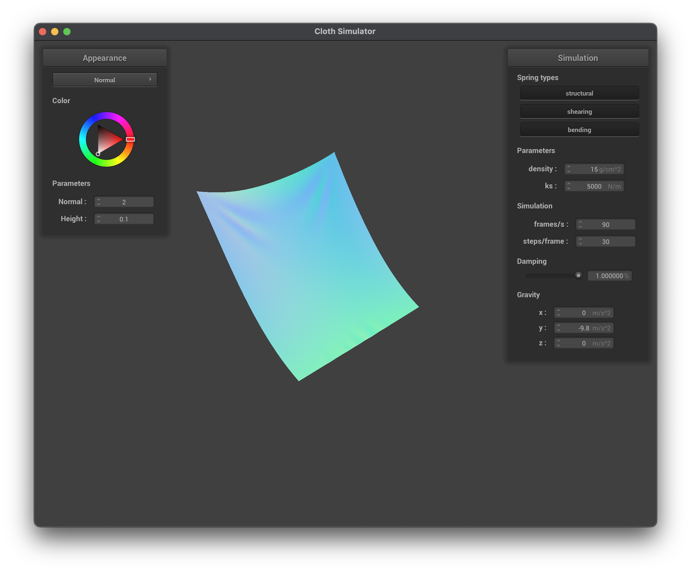
../scene/pinned2.json, damping = 1%, normal
Show us a screenshot of your shaded cloth from scene/pinned4.json in its final resting state! If you choose to use different parameters than the default ones, please list them.

../scene/pinned4.json, final state (wireframe)

../scene/pinned4.json, final state (normal)
In this task, we handle collisions with spheres by registering when a collision "occurs" (depends on sphere vs. plane) and then calculate a correction to the point mass's current position so that it is just outside the surface of the object being collided into. A collision occurs when the point mass has a distance to the center of the sphere less than its radius. If a collision occurs, we calculate the tangent point along the sphere where the collision would have occured and use that value to calculate the correction vector. When updating the point mass's position, we make sure to scale by 1 - friction when multiplying by the correction vector. We also needed to update Cloth::simulate to check for collisions between every PointMass and CollisionObject.
Show us screenshots of your shaded cloth from scene/sphere.json in its final resting state on the sphere using the defaultks = 5000as well as withks = 500andks = 50000.
ks = 5000 N/m (default)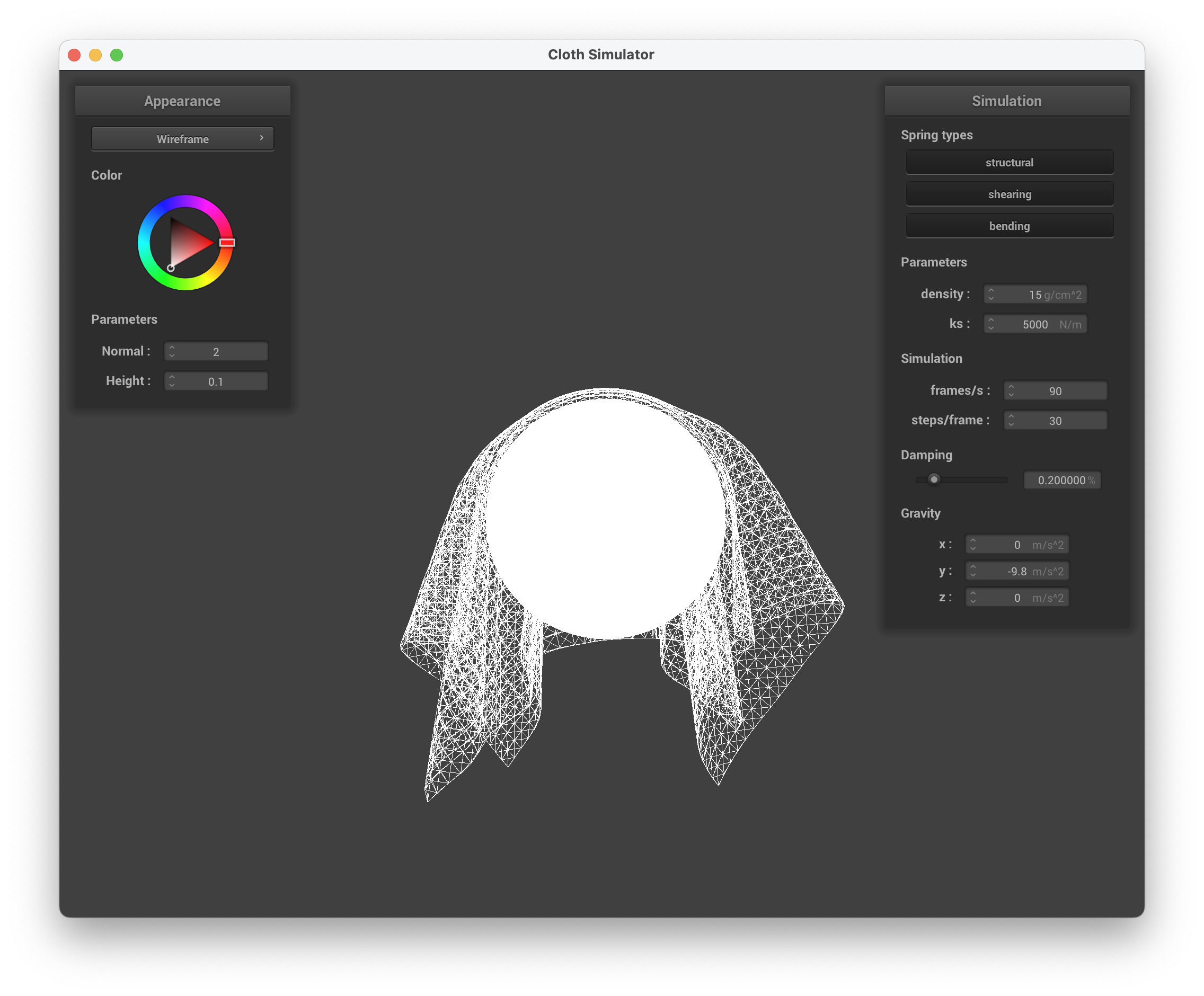
../scene/selfCollision.json, ks = 5000 N/m, wireframe
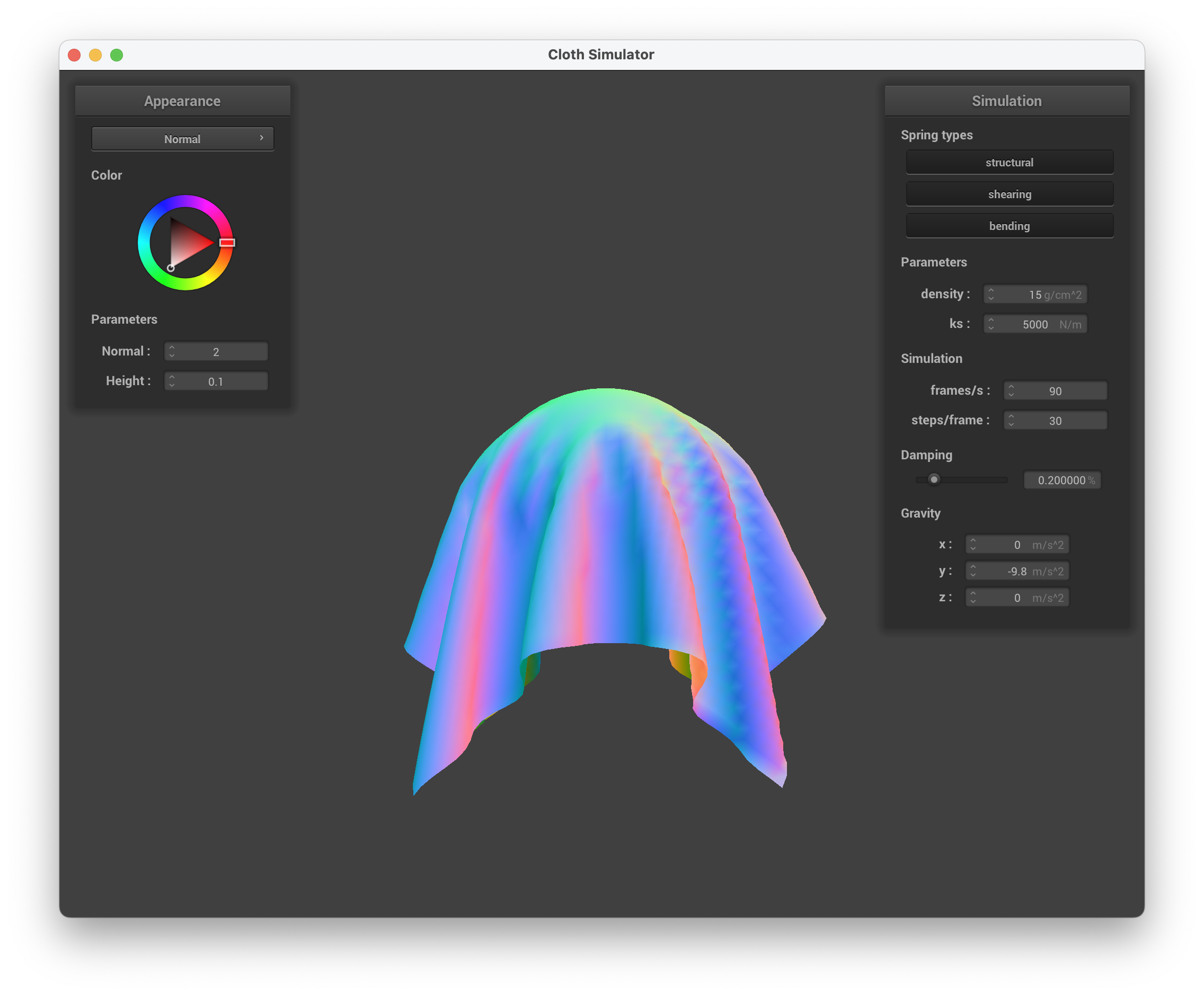
../scene/selfCollision.json, ks = 5000 N/m, normal
ks = 50 N/m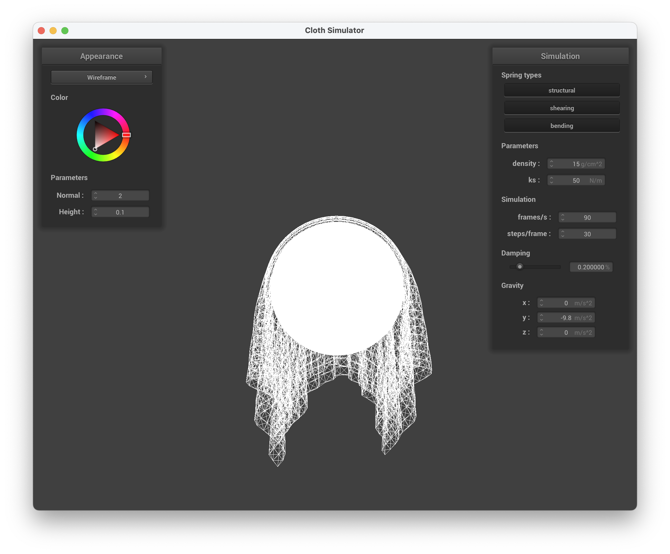
../scene/selfCollision.json, ks = 50 N/m, wireframe
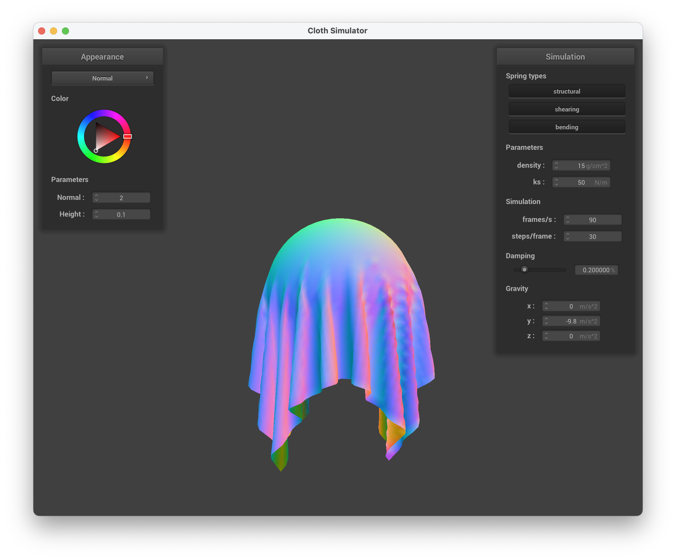
../scene/selfCollision.json, ks = 50 N/m, normal
ks = 500 N/m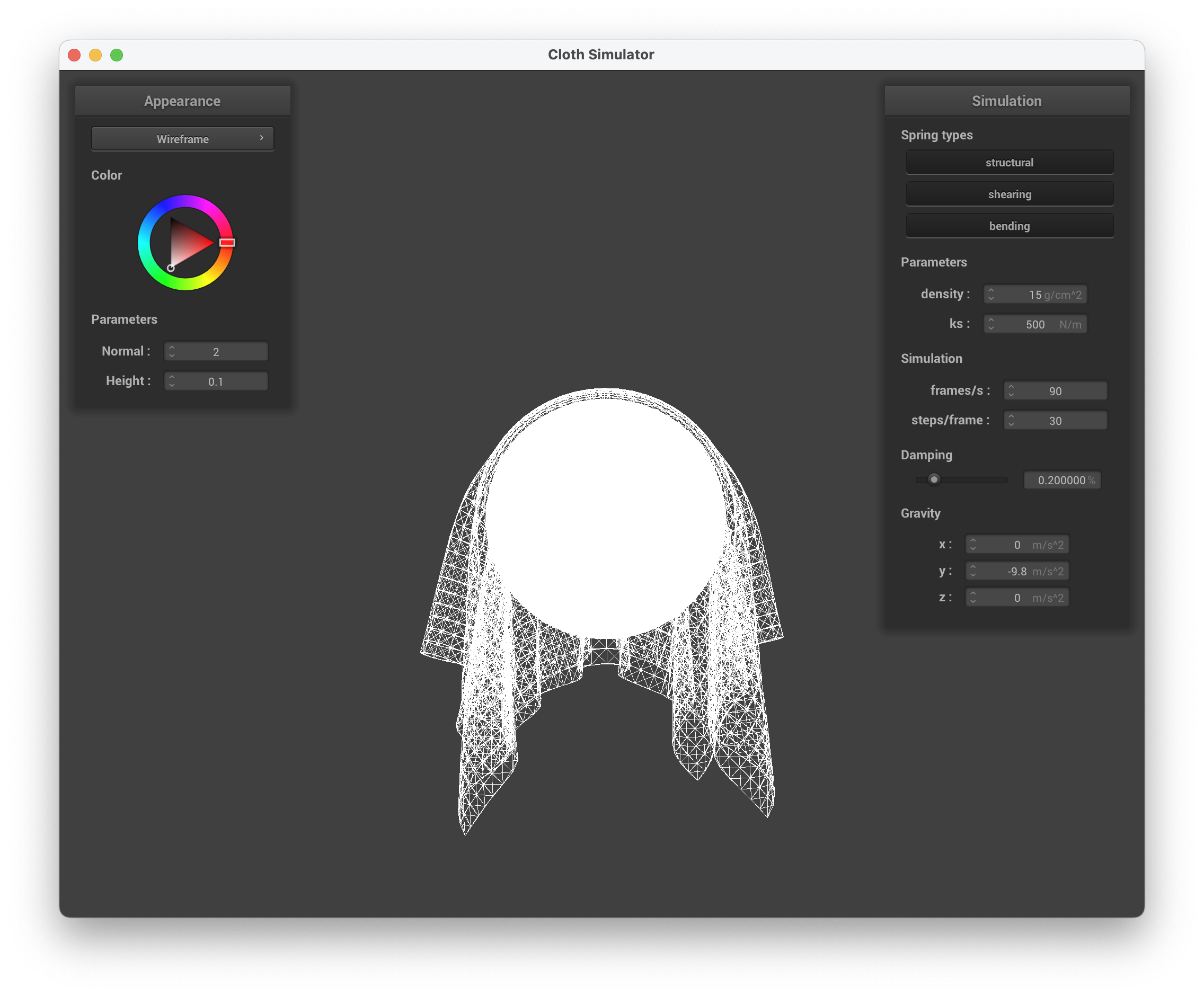
../scene/selfCollision.json, ks = 500 N/m, wireframe
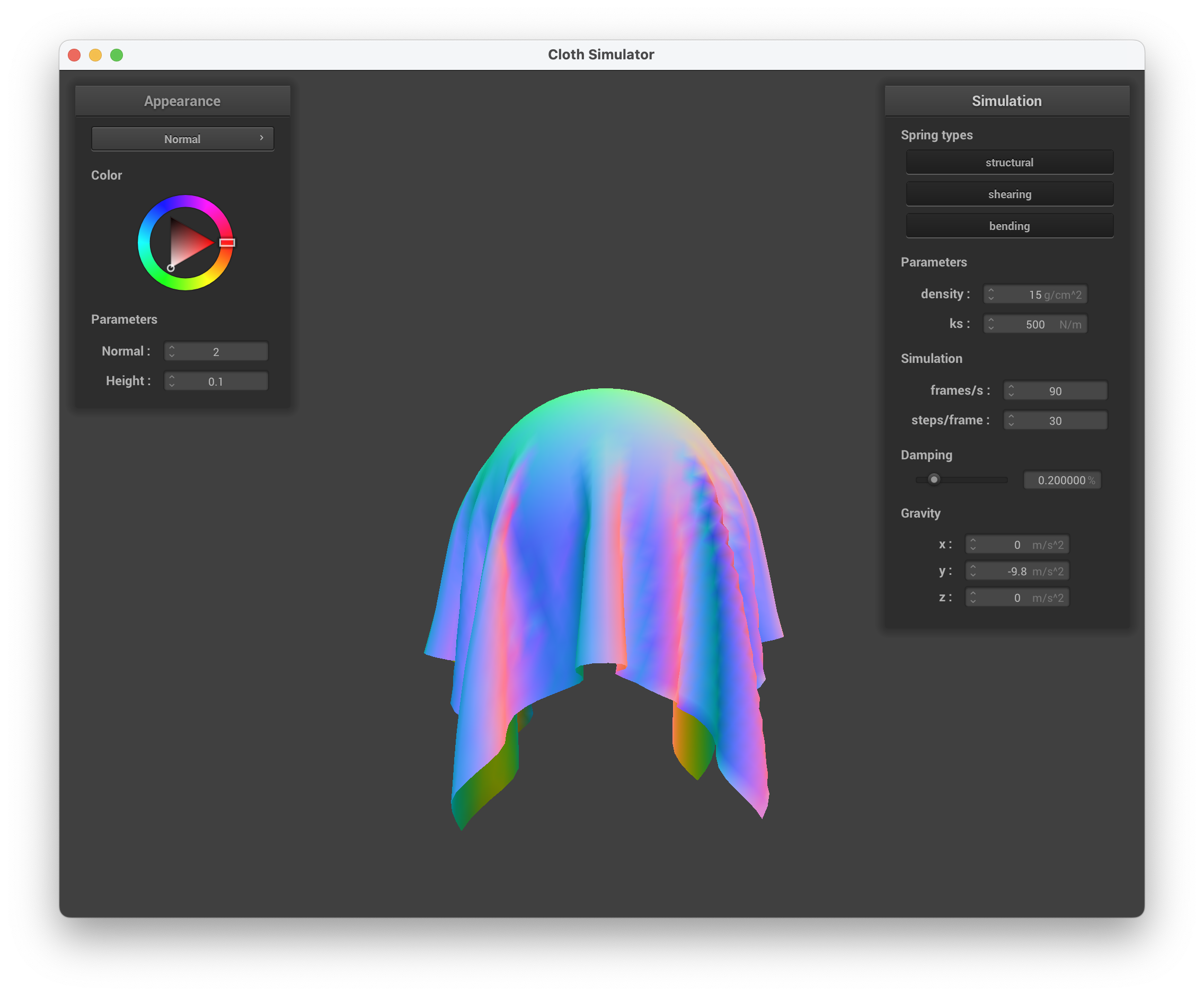
../scene/selfCollision.json, ks = 500 N/m, normal
ks = 50,000 N/m
../scene/selfCollision.json, ks = 50000 N/m, wireframe
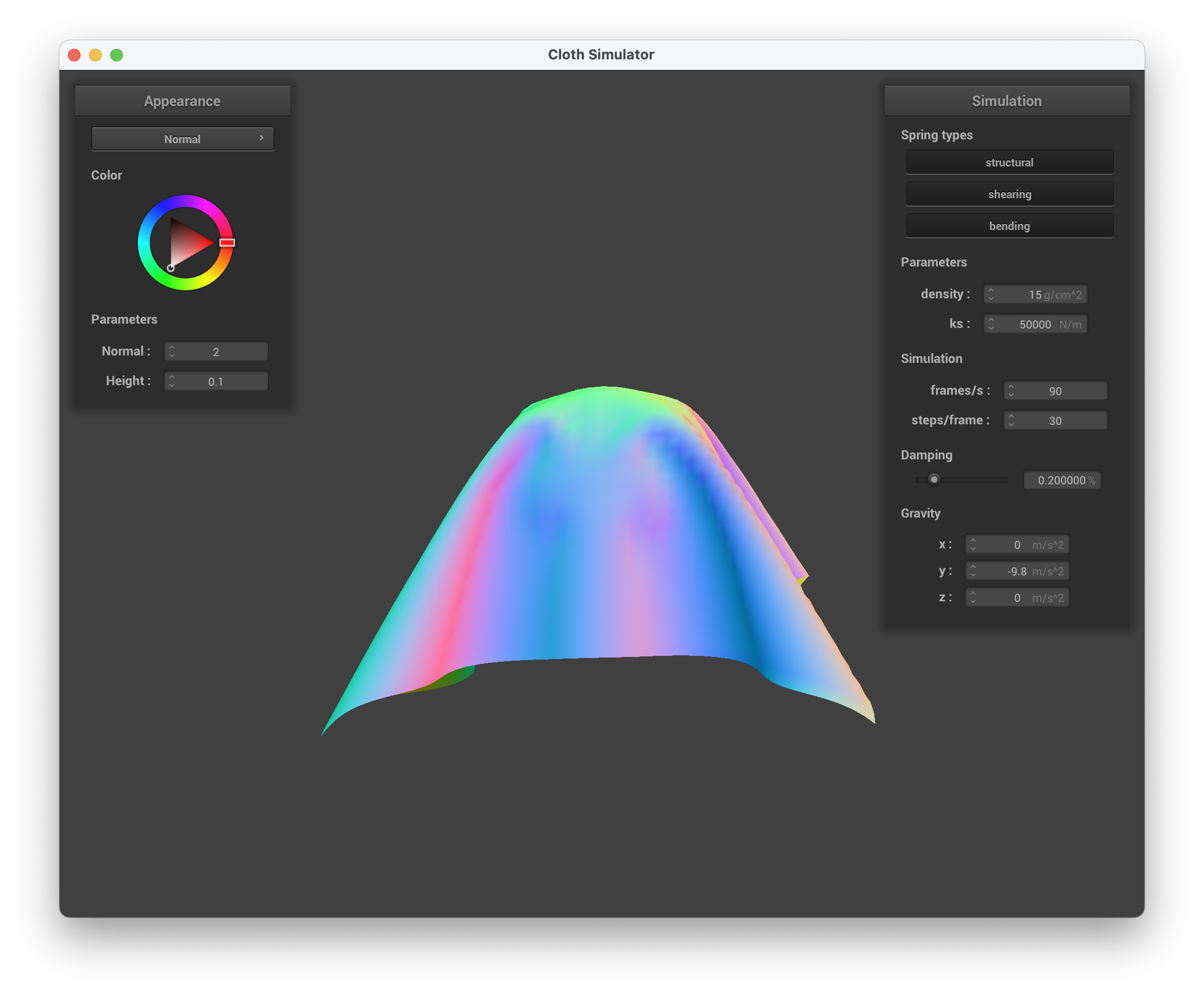
../scene/selfCollision.json, ks = 50000 N/m, normal
Describe the differences in the results.
We can see through the images below that when we increase ks, this results in increasing the stiffness of the spring. The cloth becomes more rigid and there is more structure to the folds. The material also goes from looking like velvet/silk to a stiffer material. This makes sense because a stiff spring will resist the deformation from gravity. In contrast, at lower ks values, the cloth is more flexible because of a weaker spring, hence why it appears more "loose" and drapes easier. This is especially prevalent when ks = 50 N/m, where the cloth resembles a thin hankerchief/napkin.
In this task, we handle collisions with planes - for a plane, a collision occurs when the point mass has crossed the plane. We determine if a point had crossed the plane by checking if the dot product of the movement vector and the normal vector is negative. If so, we apply a correction which uses the tangent point at which the collision between the point mass and the plane would have occurred. We also needed to factor in SURFACE_OFFSET when multiplying by the normal vector. The correction vector is also similar to collisions with a sphere. Lastly, we also needed to update Cloth::simulate to check for collisions between every PointMass and CollisionObject.
Show us a screenshot of your shaded cloth lying peacefully at rest on the plane. If you haven't by now, feel free to express your colorful creativity with the cloth! (You will need to complete the shaders portion first to show custom colors.)
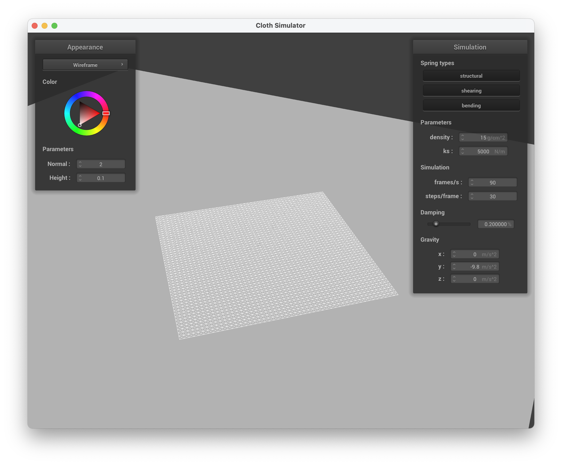
../scene/plane.json, wireframe
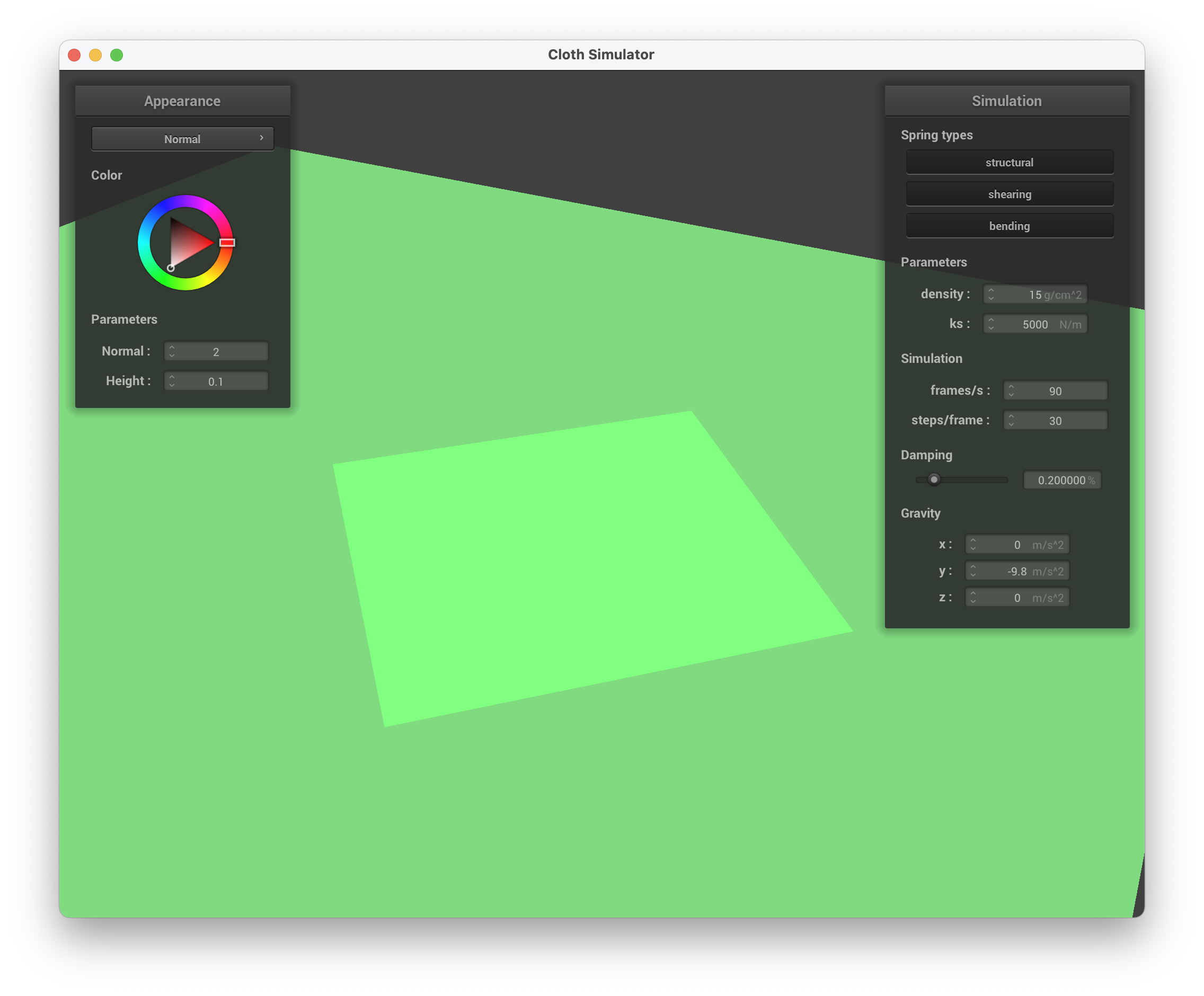
../scene/plane.json, normal
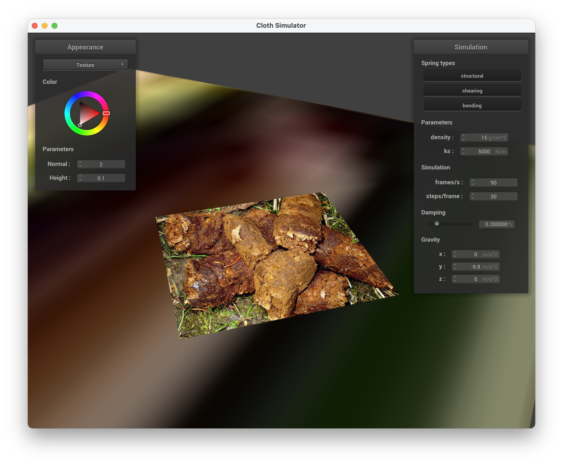
../scene/plane.json, custom texture of poop
Prior to this section, our cloth when colliding with itself would just clip through itself. To prevent this, we would need to implement that whenever the cloth fell on itself, it would fold. For each point mass, we need to check whether it is within some small number (2 * thickness) away from another point (not including itself). If it is too close, then we apply a correction/repulsive collision force (to maintain a minimum of 2 * thickness distance away).
Cloth::hash_position
In this task, we implemented Cloth::hash_position which takes in a point mass's position and calculates its 3D box volume's index in our spatial hash table. The idea is to check within a point's 3D box volume instead of throughout the entire cloth. This was done by first calculating its 3D position (w, h, t) where w = 3 * width / num_width_points, h = 3 * height / num_height_points, and t = max(w, h). We determined the 3D box coordinates by calculating x = (pos.x - fmod(pos.x, w))/w, y = (pos.y - fmod(pos.y, h))/h, and z = (pos.z - fmod(pos.z, t))/t. Afterwards, we transformed the 3D position to 1D through our hash expression.
Cloth::build_spatial_map
In this task, we constructed our spatial map by iterating through all point_masses in the cloth and calculated its hash. If there isn't already a vector at that position, a new one is initialized and we also push_back the current point mass.
Cloth::self_collide
In this task, we check each point mass to see whether the normalized distance between it and candidate point masses is less than 2 * thickness. If a collision is detected, a correction vector is calculated based on the difference between the desired separation distance (2 * thickness) and the actual distance between the point masses.
If any corrections were calculated, the average correction vector is computed and the position of the given point mass is adjusted by adding the correction vector to it.
We also needed to update Cloth::simulate to build our spatial map and iterate through the point masses to call self_collide on them.
Show us at least 3 screenshots that document how your cloth falls and folds on itself, starting with an early, initial self-collision and ending with the cloth at a more restful state (even if it is still slightly bouncy on the ground).
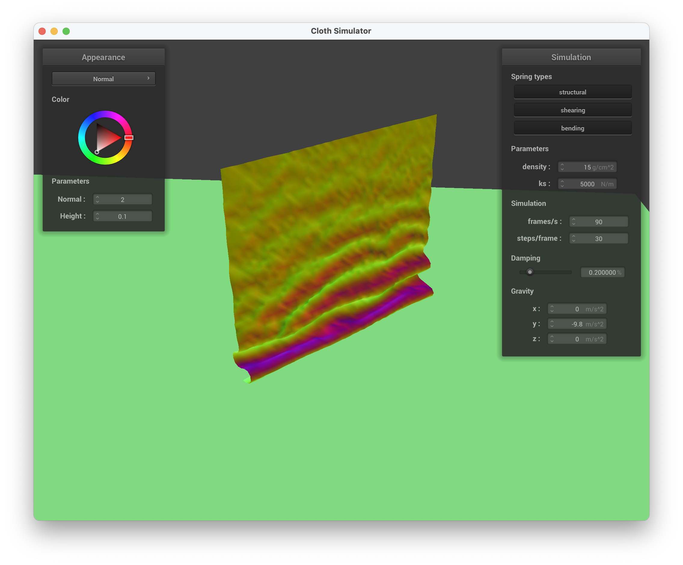
../scene/selfCollision.json, early, initial self-collision
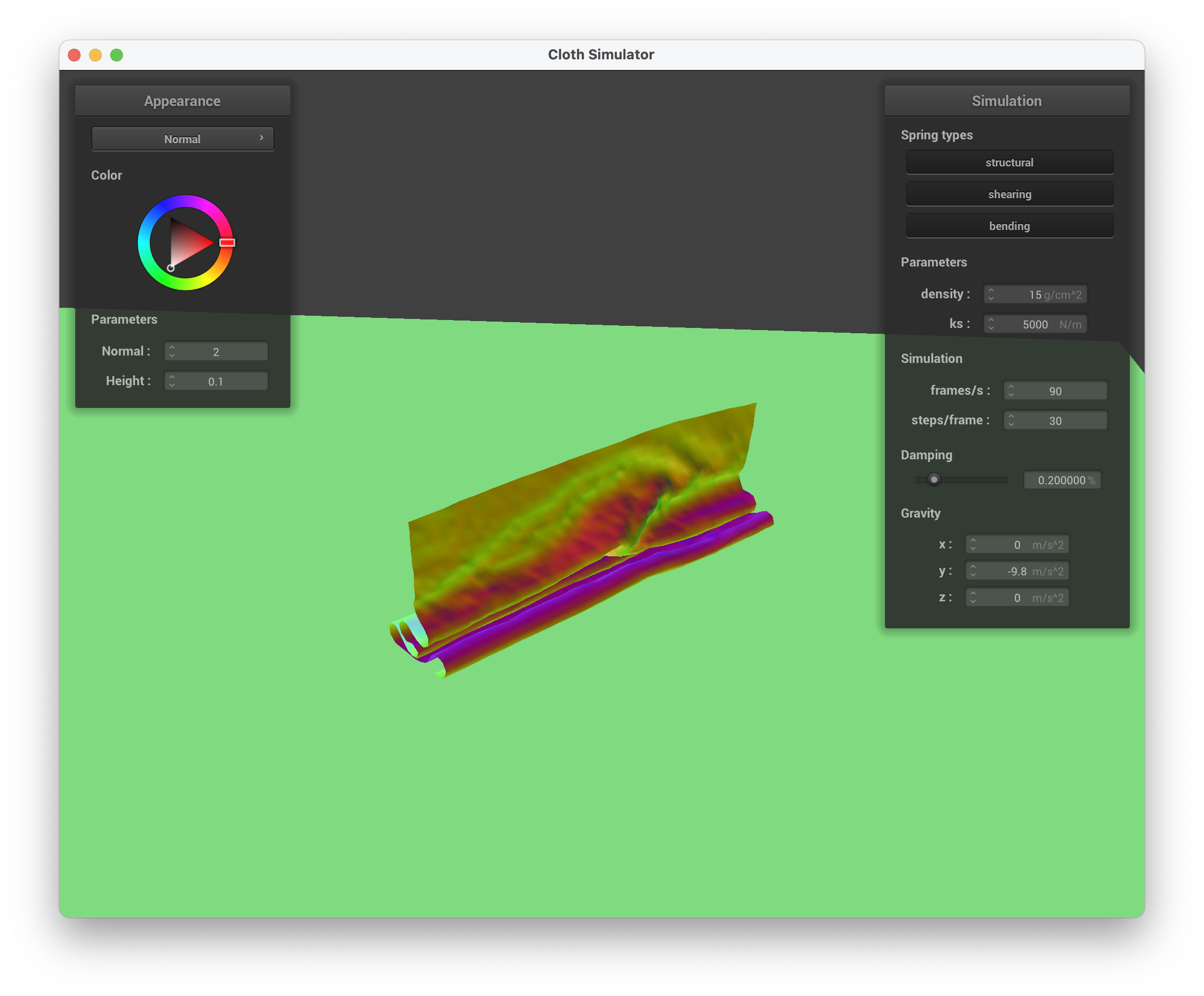
../scene/selfCollision.json, continuing to fall down
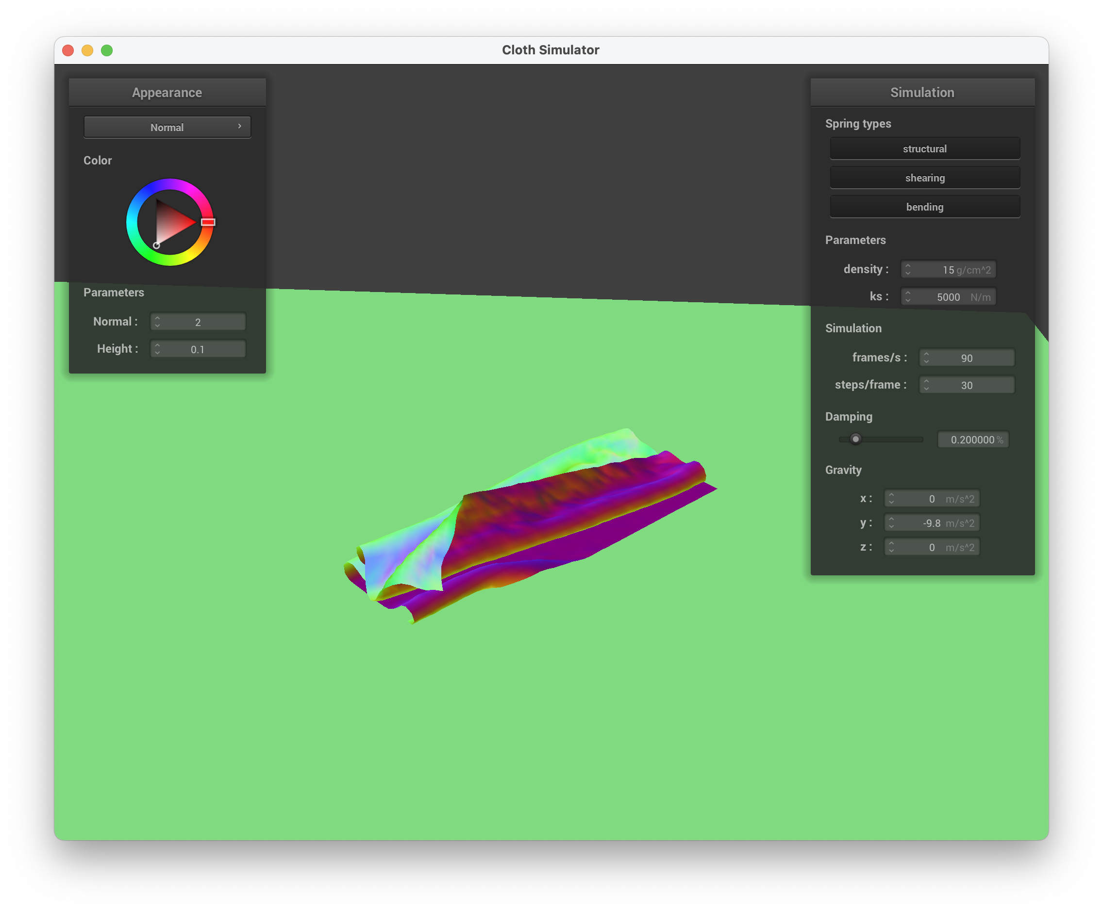
../scene/selfCollision.json, down with more folds
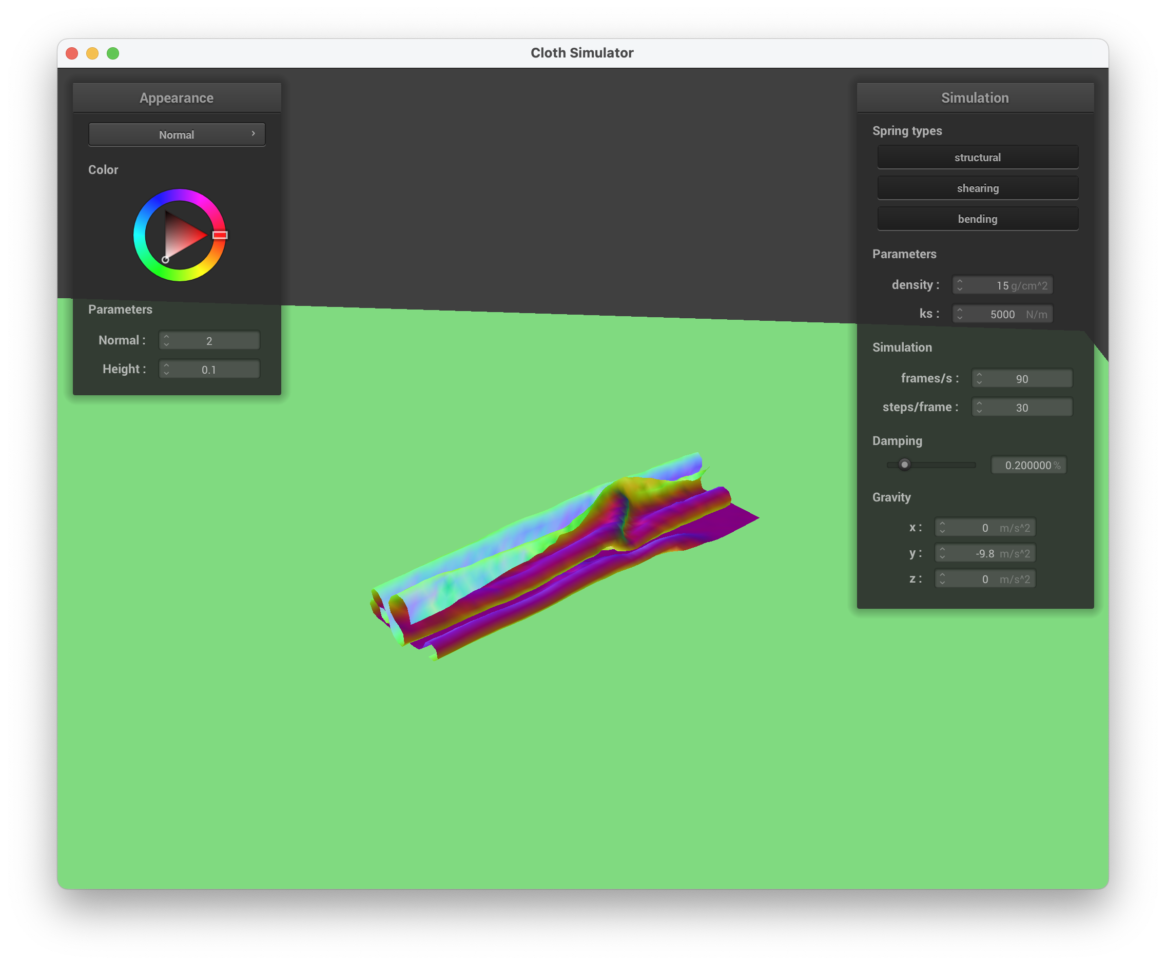
../scene/selfCollision.json unravelling

../scene/selfCollision.json, continuing to unravel itself
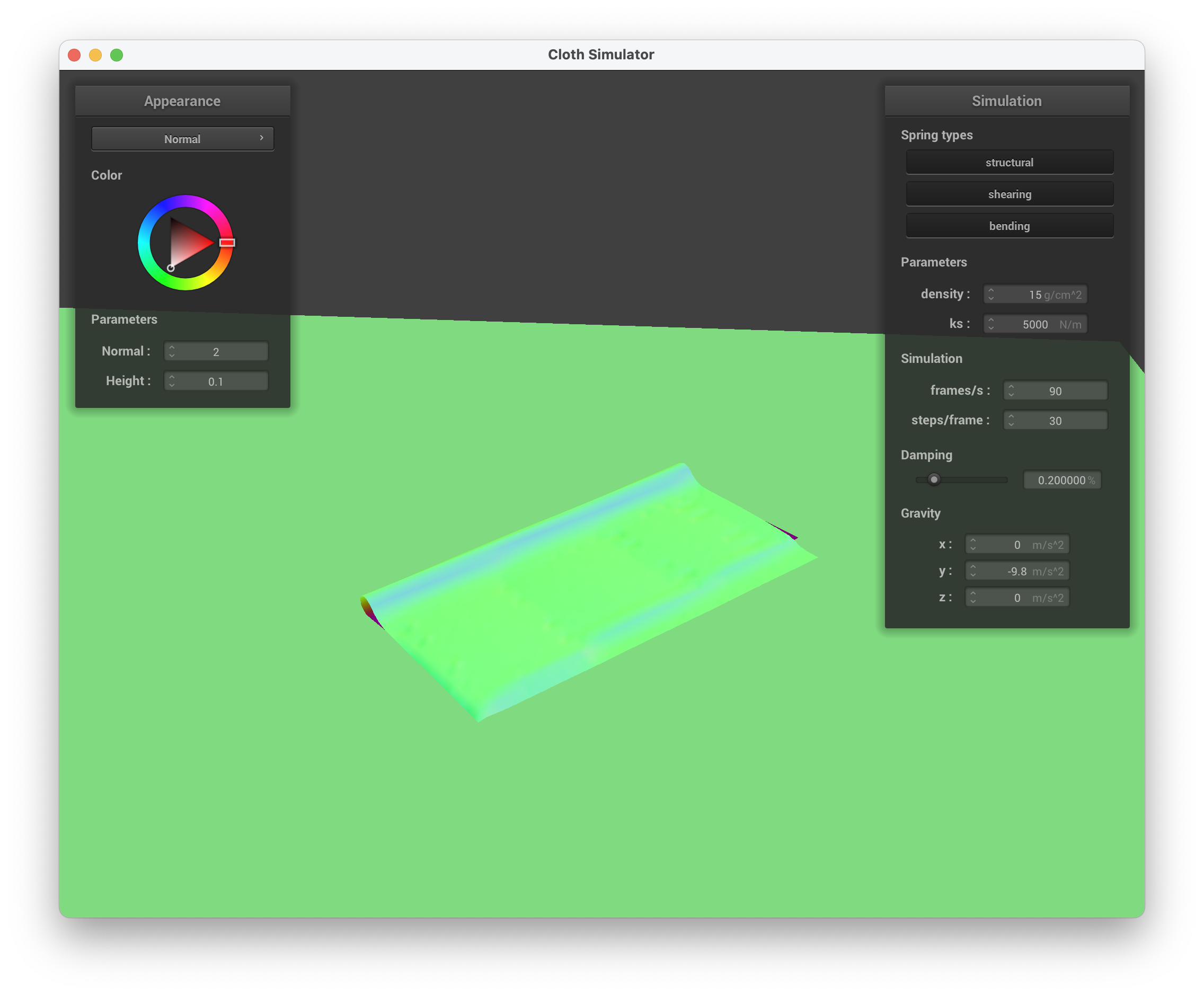
../scene/selfCollision.json, final resting state
Vary thedensityas well asksand describe with words and screenshots how they affect the behavior of the cloth as it falls on itself.
ks
When maintaining the default parameters (density, damping) and only modifying the spring constant, ks, we can see that at a lower ks value (ks = 50 N/m), the cloth has a bunch of folds, similar to a piece of aluminum foil or tissue paper. The ripples are very small and there are a bunch of self collisions, which makes sense intuitively since the spring constant is smaller. With a lower ks, the cloth is more malleable/flexible since it has less structure. We can compare this to ks being a greater value — when ks = 50,000 N/m, there are less folds ("bigger" folds compared to when ks = 50 N/m) and the strength of the cloth is greater due to the higher spring constant.
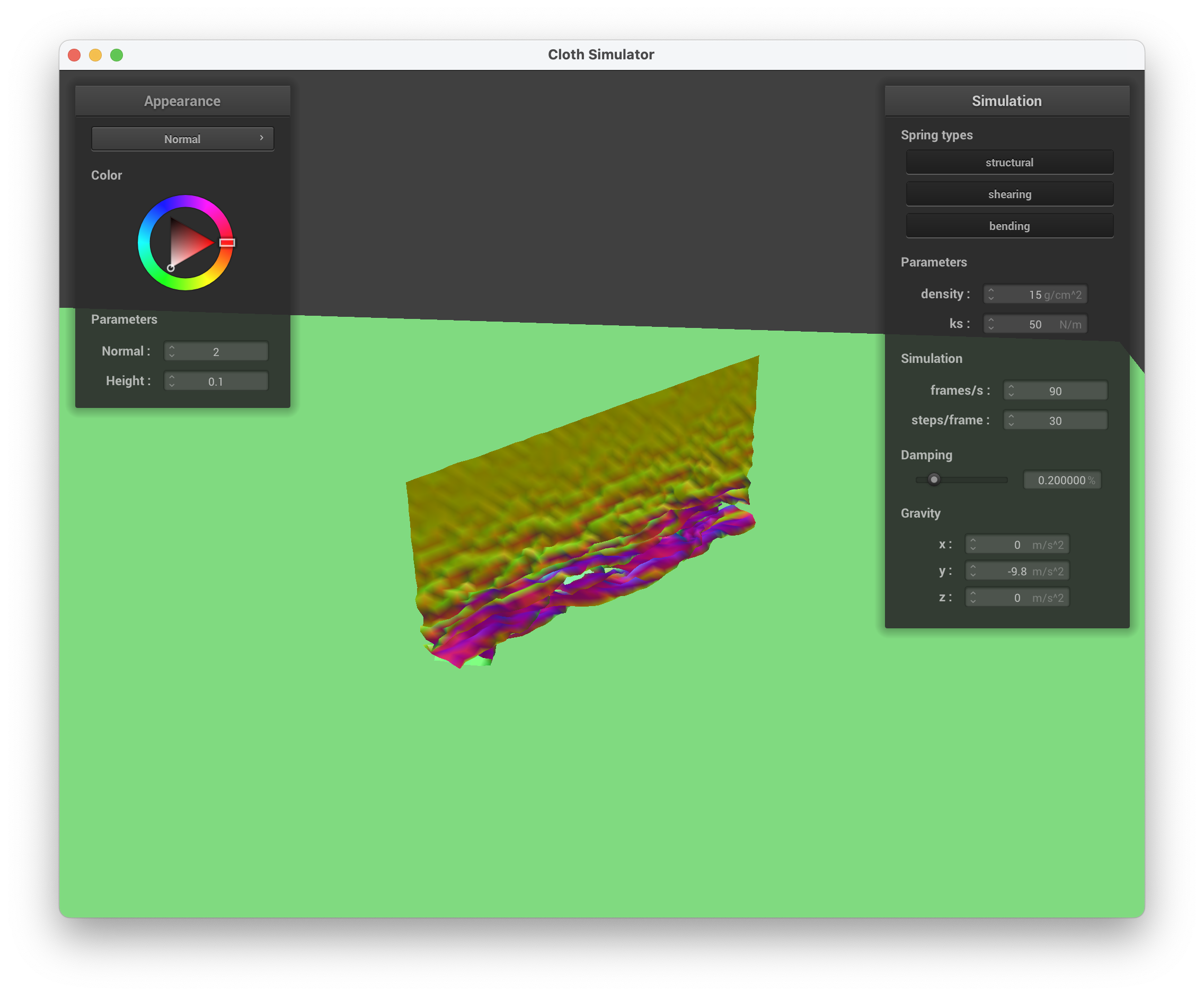
../scene/selfCollision.json, ks = 50 N/m, very small waves
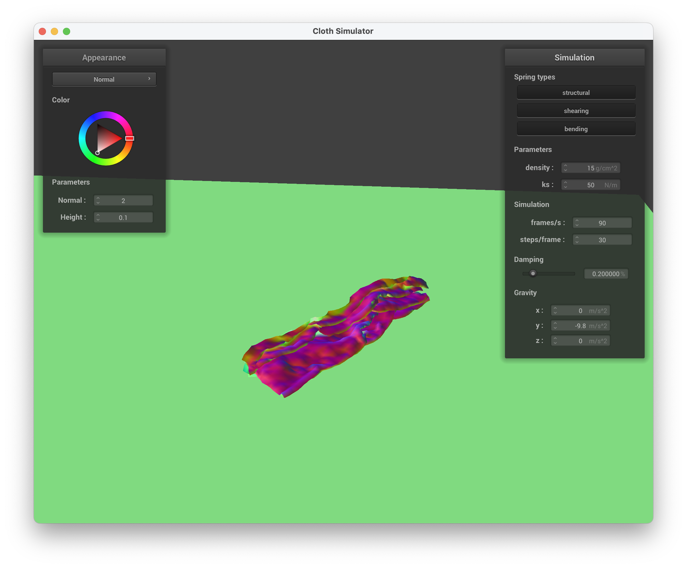
../scene/selfCollision.json, ks = 50 N/m, with many self-collisions/ripples
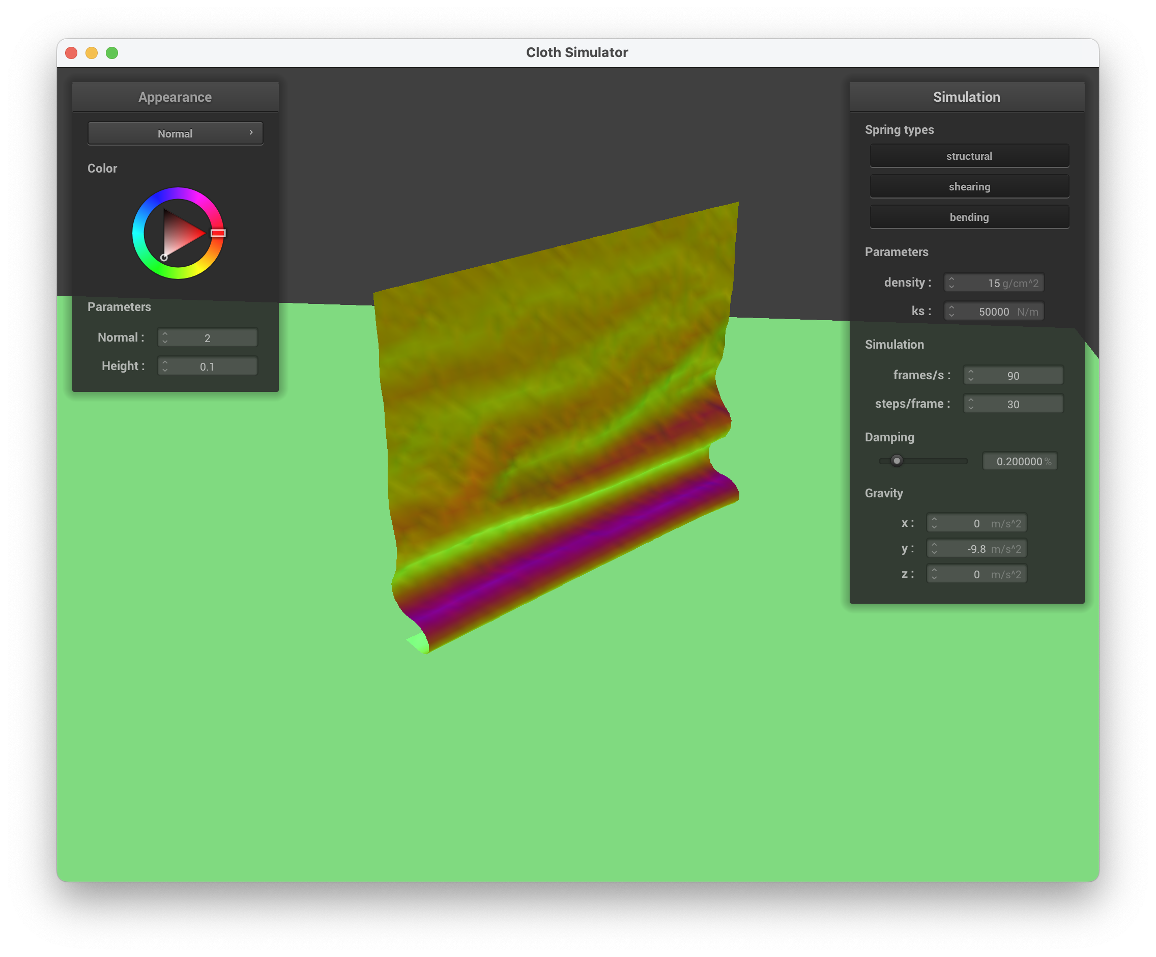
../scene/selfCollision.json, ks = 50,000 N/m, much larger waves
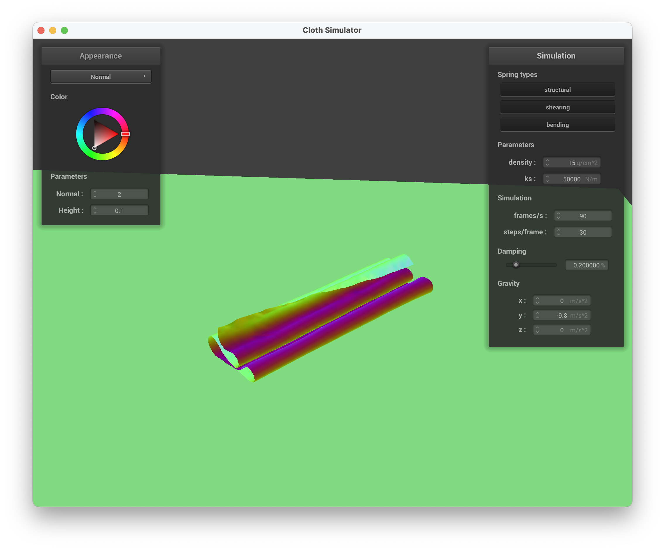
../scene/selfCollision.json, ks = 50,000 N/m, larger folds as it begins to settle
density
When maintaining the default parameters (ks, damping) and only modifying the density, we can see that at a lower density (density = 1 g/cm^2), the cloth mimics gift wrapping paper in the way it folds (and its appearance). This makes sense because paper generally has low density and doesn't "bunch up" together. A lower density equates to a lower mass, hence why there is less force applied and less self collisions. In contrast, at a higher density, there is greater mass so a larger force is applied to the cloth, causing more self-collisions. This is depicted when density = 50 g/cm^2, where the cloth has more folds/ripples (less able to hold its structure) and appears "heavier" like a blanket.
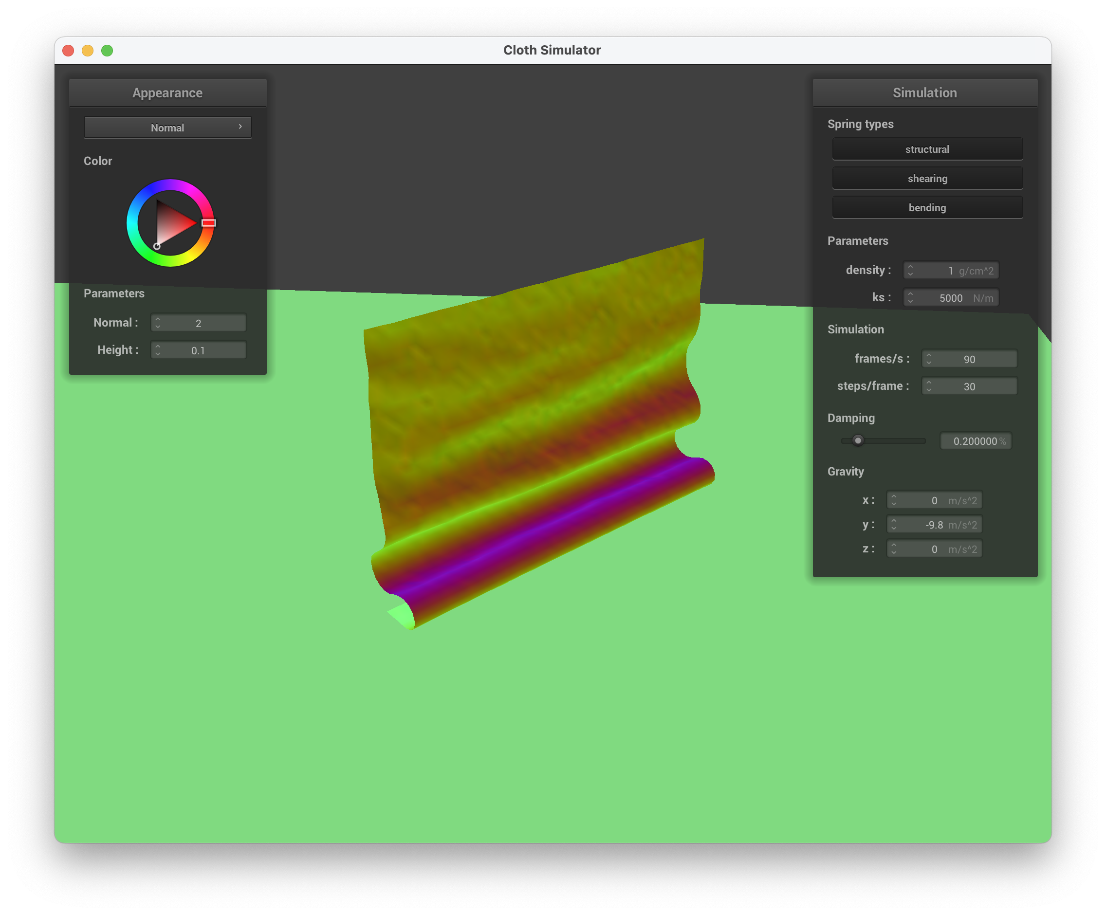
../scene/selfCollision.json, density = 1 g/cm^2, beginning to fold over
../scene/selfCollision.json, density = 1 g/cm^2, slowly unravelling
../scene/selfCollision.json, density = 50 g/cm^2, many small ripples
../scene/selfCollision.json, density = 50 g/cm^2, still falling down with more ripples/folds
Explain in your own words what is a shader program and how vertex and fragment shaders work together to create lighting and material effects.
For this part, we are creating various shaders using the language GLSL. A shader program is used to make rendering more efficient/faster by transferring rendering workload from the CPU to the GPU (processes the vertex and fragments in the rasterization pipeline). Two shader types — vertex and fragment — work together to create the lighting and material effects that we want. The vertex shader deals with the position and transforms of the vertices themselves (from the 3D positions to 2D screen space based on the camera position and perspective). After processing the vertex positions, it will save the final vertex position. The output of the vertex shader is inputted into the fragment shader, which essentially just calculates the final color to be outputted after factoring in lighting, textures, and material properties. It does this by reading the geometric attributes passed in, and doing the appropiate calculations to get the exact color to be outputted by that fragment. The combination of these two shaders allows for the creation of realistic images in a computationally efficient approach.
In this task, we implemented diffuse shading, which is related to Lambert's Law. To implement this, we used the equation given in lecture: we first found the dot product between the normal vector and the direction vector of the light. We ensured that it was a positive number, then multiplied it with the light intensity to get the final out color that we need.
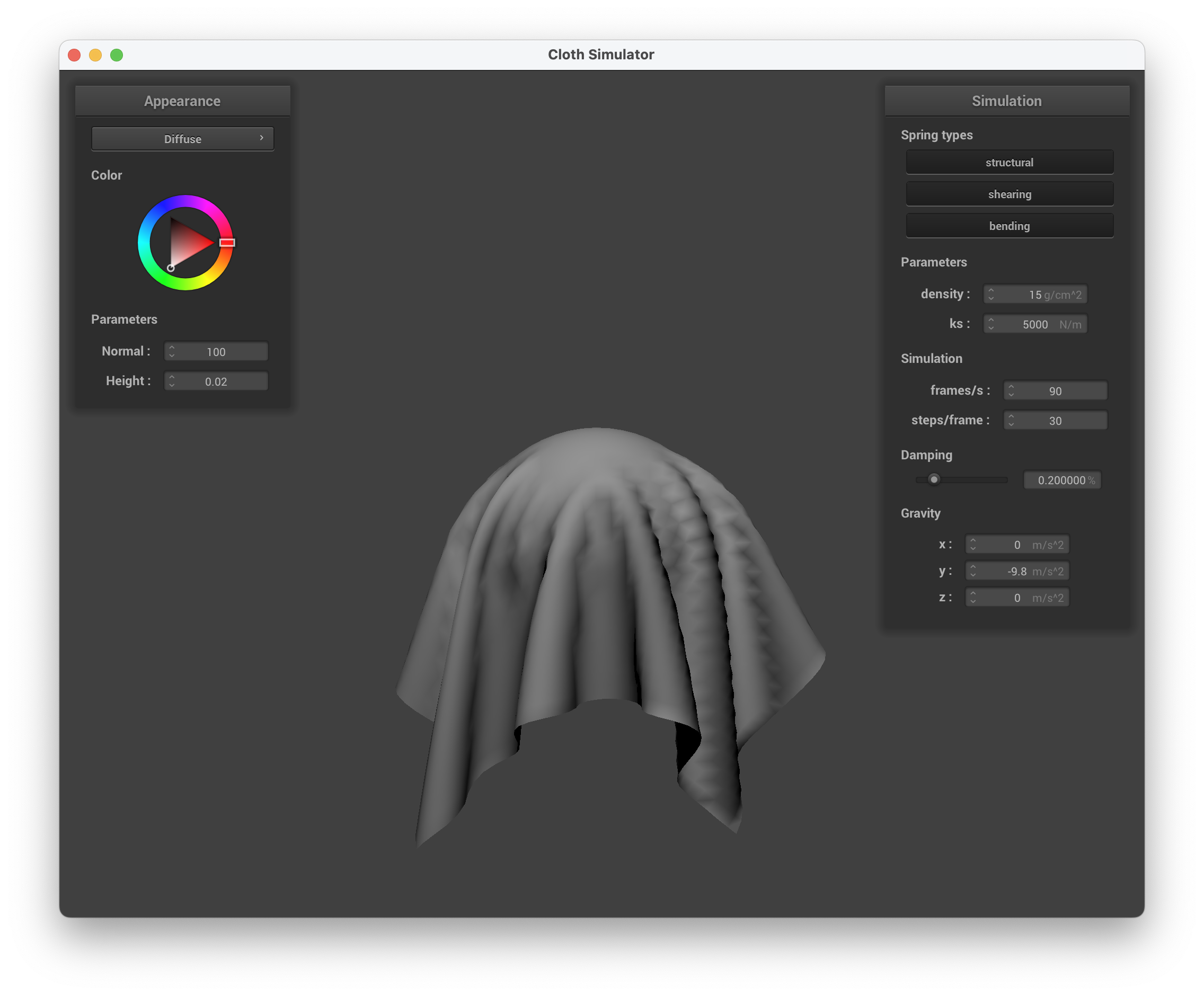
../scene/sphere.json, diffuse shading
Explain the Blinn-Phong shading model in your own words. Show a screenshot of your Blinn-Phong shader outputting only the ambient component, a screen shot only outputting the diffuse component, a screen shot only outputting the specular component, and one using the entire Blinn-Phong model.
The Blinn-Phong shading model essentially takes in three different aspects — ambient, diffuse, and specular — and adds them together to create the final shader. The ambient shading accounts for the constant color without any other factors involved. The diffuse shading accounts for the light and how it interacts with the curve of the object, but it is independent of the view direction. The specular shading accounts for view direction, adding in the intensity of the light based on that. Adding together these three components creates a very realistic shader, accounting for the different parts of the environment.
In this task, we implemented these three parts to create the final Blinn-Phong shader. For the diffuse shader, we took the code from Task 1 of this part. For the ambient portion, we simply added the input color itself. For the specular portion, we wanted an effect similar to a mirror. Instead of using the regular normal vector, we used the bisector vector of the light and view vectors. This way, it would depend on the view direction as we want. Finally, we just added all three of these parts to get the final out color.
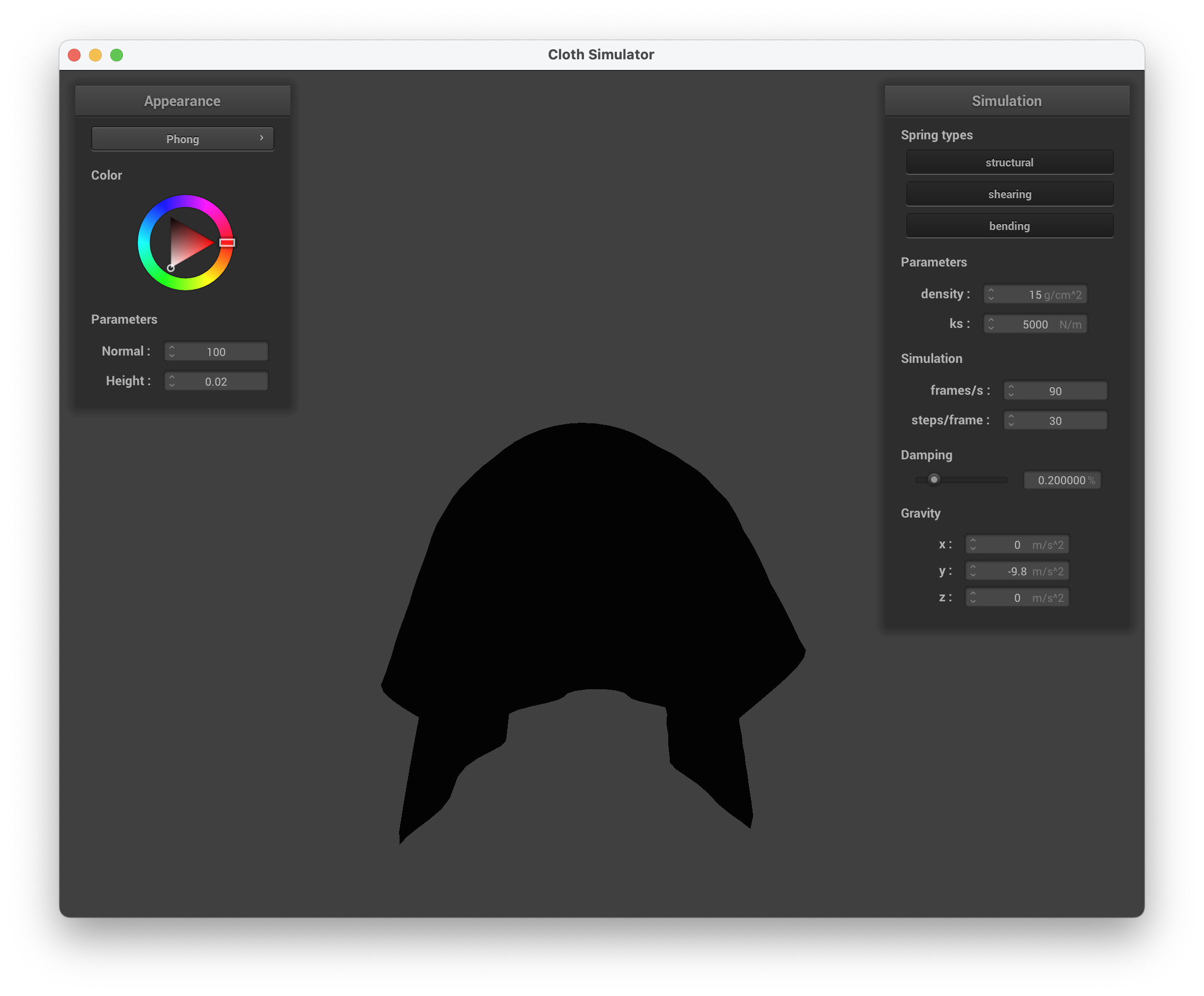
../scene/sphere.json, ambient component only
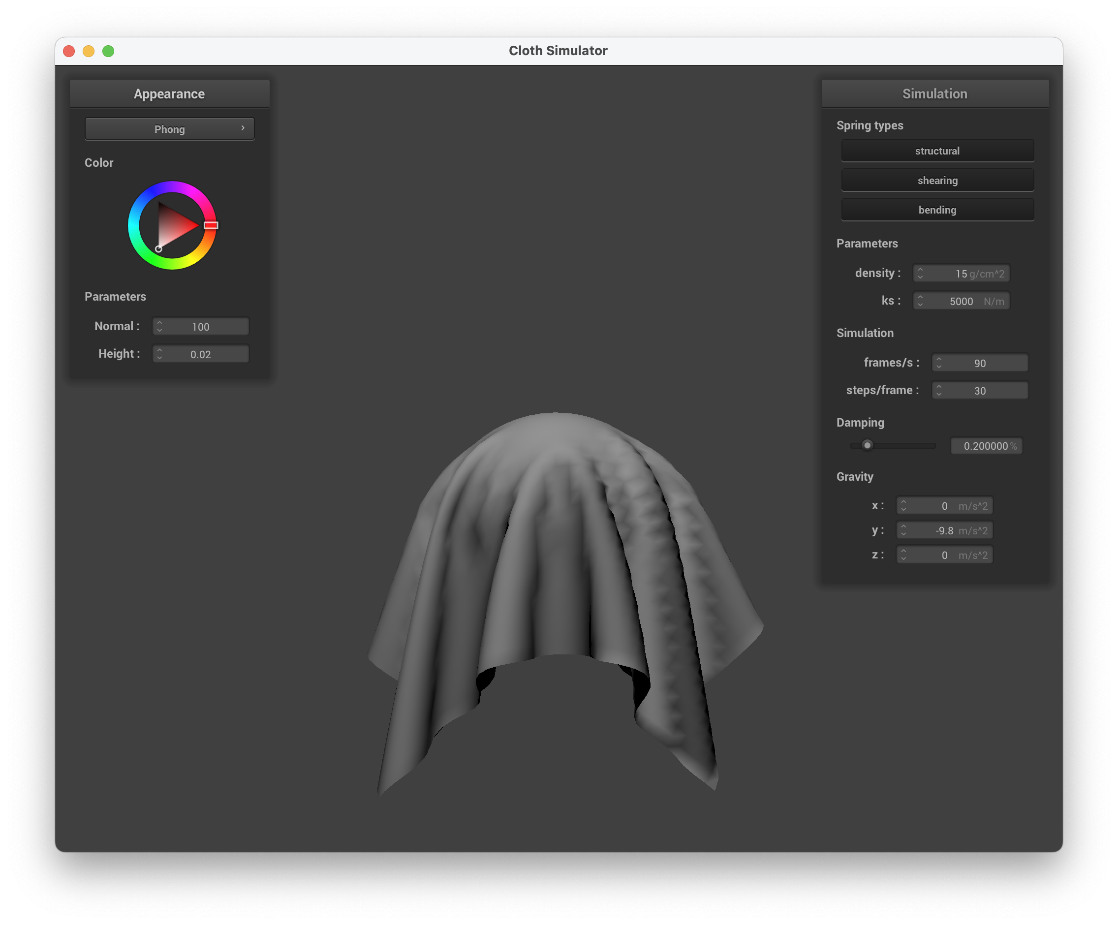
../scene/sphere.json, diffuse component only
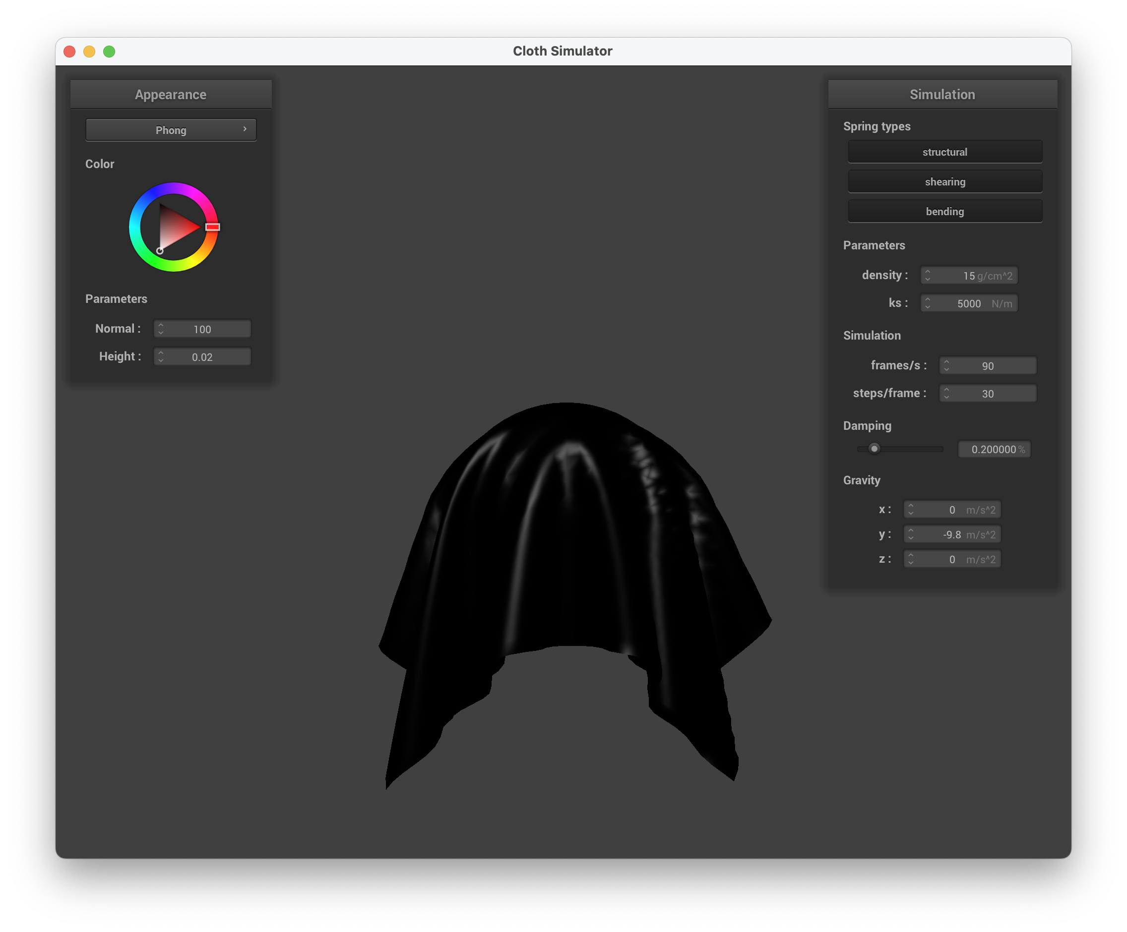
../scene/sphere.json, specular component only
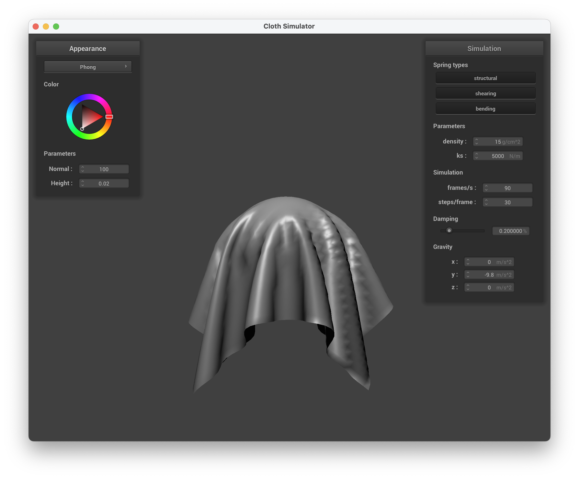
../scene/sphere.json, complete Blinn-Phong model
In this task, we wanted to create a shader that maps a given texture to the object. We implemented this taking advantage of the texture() function in GLSL that allows us to sample from the given texture at a certain location. Using this, we can get our final out color needed.
Show a screenshot of your texture mapping shader using your own custom texture by modifying the textures in /textures/.
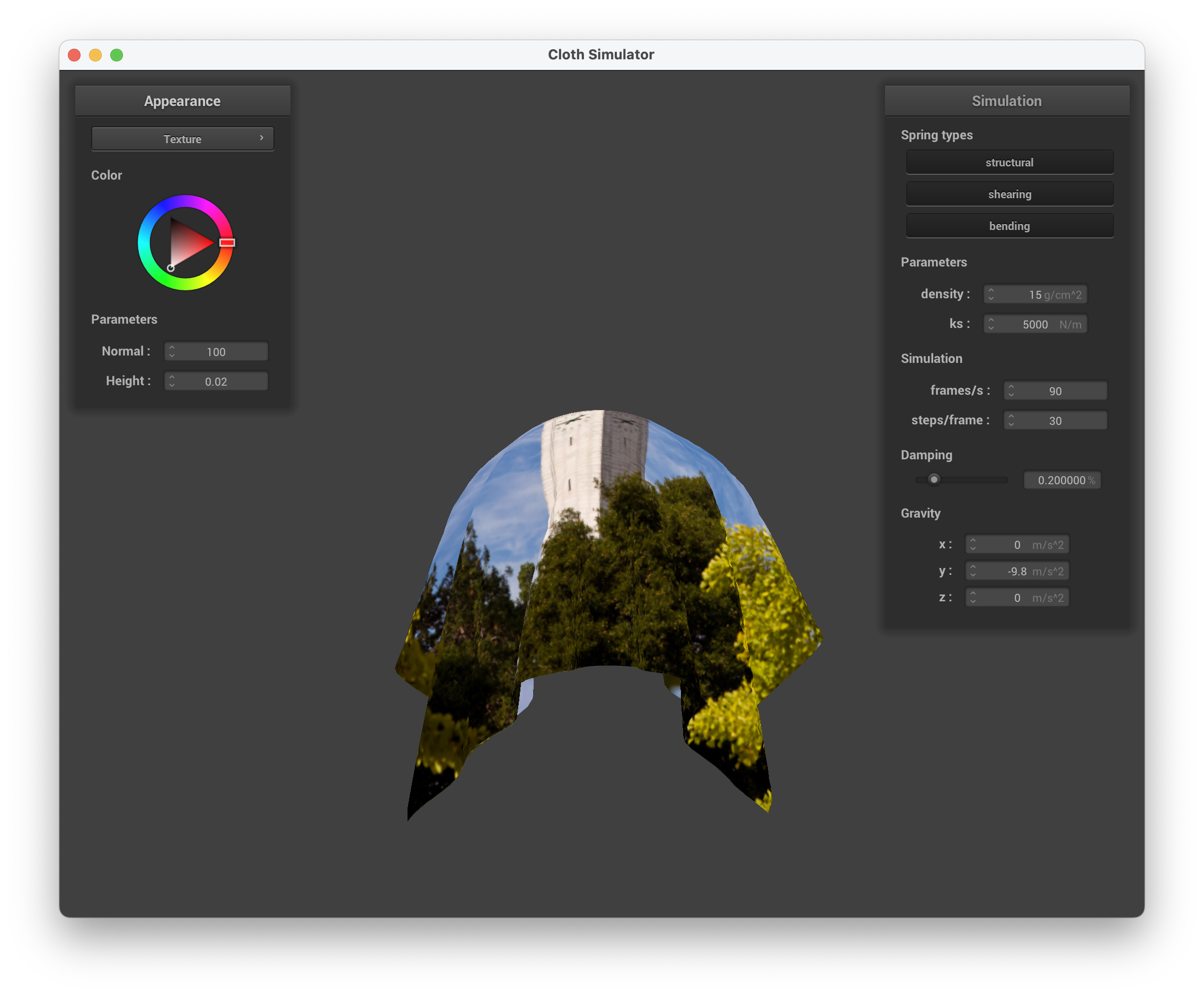
../scene/sphere.json, default Campanile texture shader
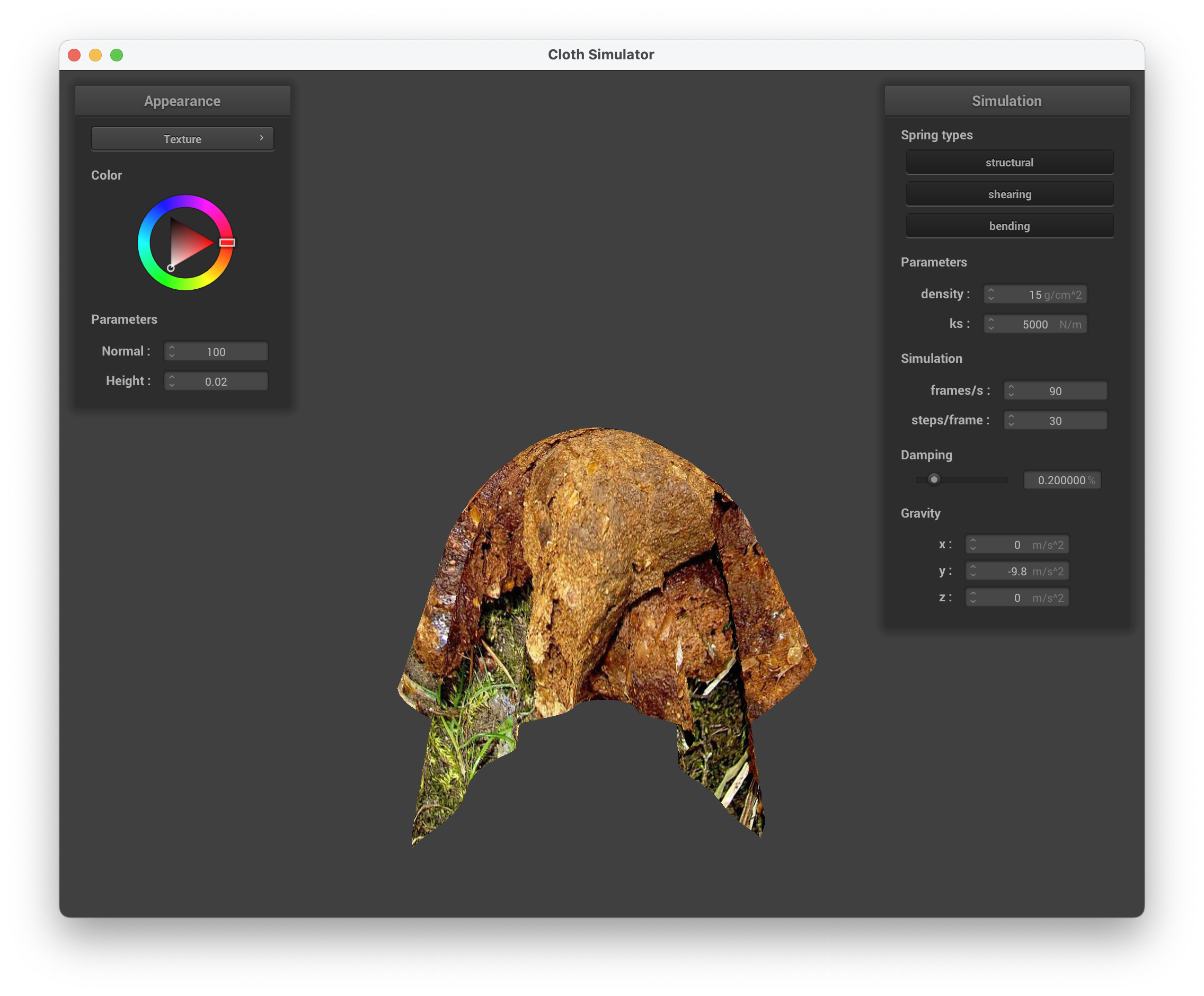
../scene/sphere.json, custom texture shader
Show a screenshot of bump mapping on the cloth and on the sphere. Show a screenshot of displacement mapping on the sphere. Use the same texture for both renders. You can either provide your own texture or use one of the ones in the textures directory, BUT choose one that's not the defaulttexture_2.png. Compare the two approaches and resulting renders in your own words. Compare how your the two shaders react to the sphere by changing the sphere mesh's coarseness by using-o 16 -a 16and then-o 128 -a 128.
In this task, we implemented shaders that account for bumps and displacement. For the bump mapping, we used a height map to calculate a new normal vector at a certain point, and used that vector for the Blinn-Phong shading instead of the original normal. To calculate this new normal, we look at how the height changes using the height map. We used the r component of the color to figure this out, and used the vector position as well as height and normal scalars to find the final normal vector.
Below are screenshots of running ./clothsim -f ../scene/sphere.json with bump mapping, setting the normal to 5 and height to 1, using texture3.png.
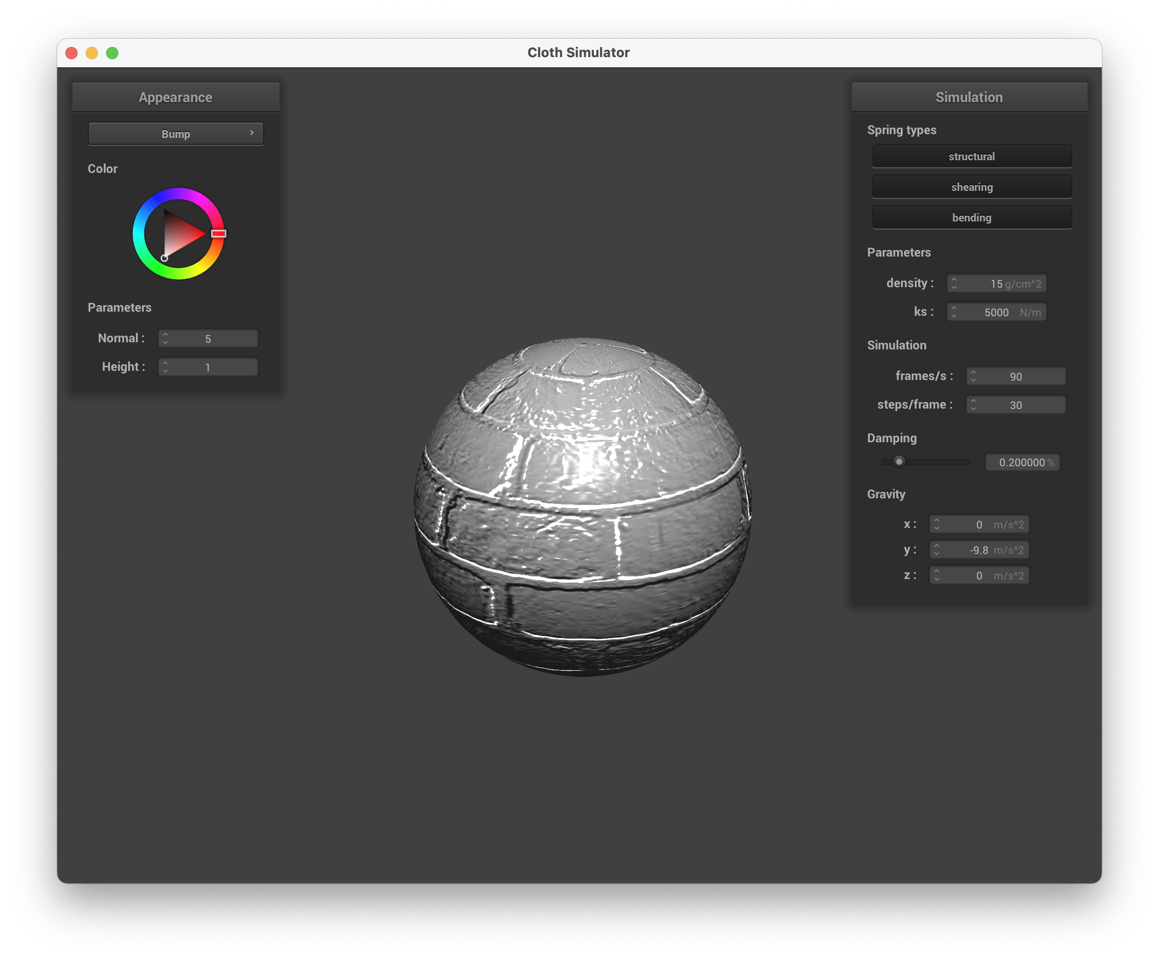
../scene/sphere.json, Bump Mapping on the Sphere
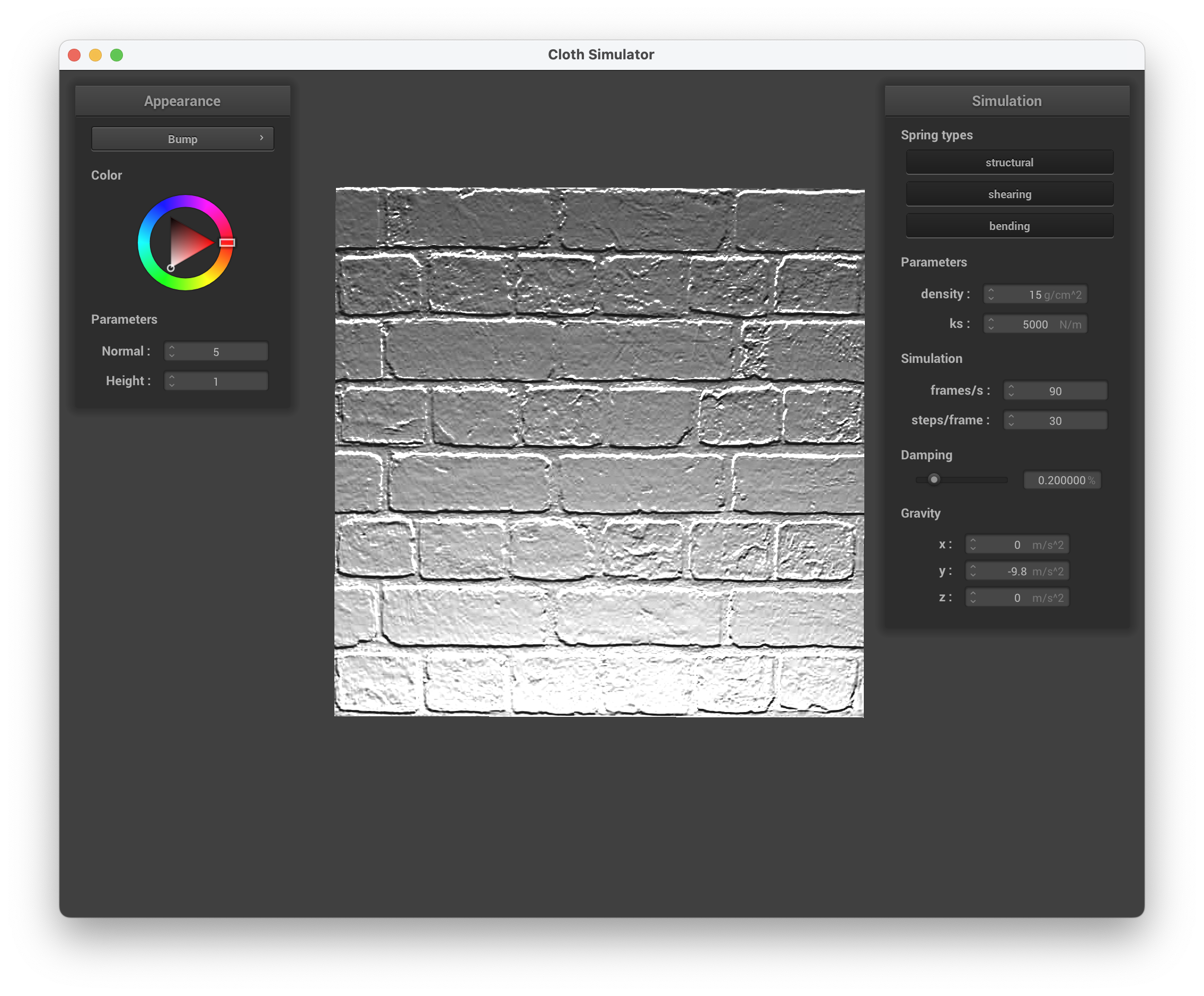
../scene/sphere.json, Bump Mapping on the Cloth
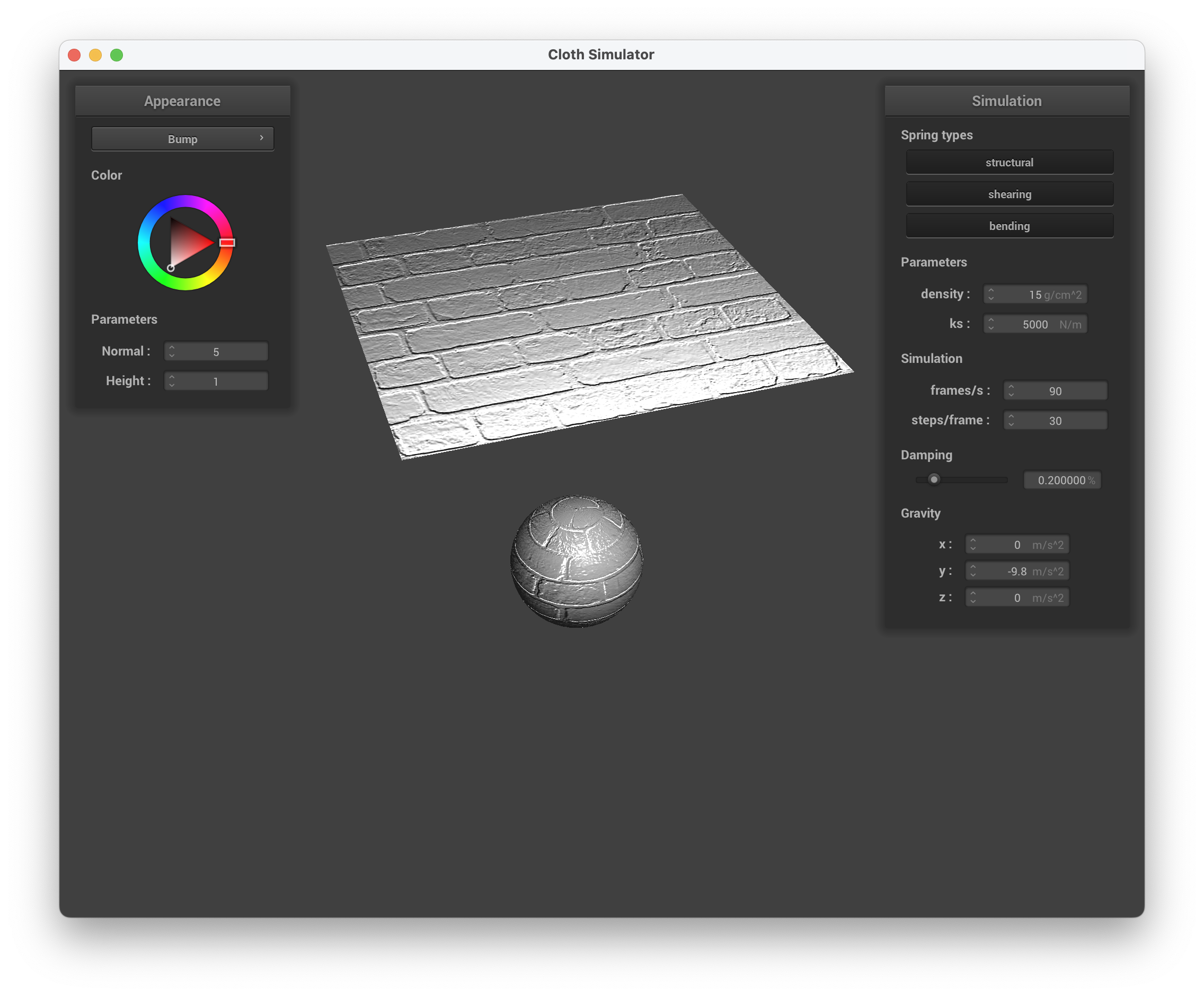
../scene/sphere.json, Bump Mapping on the Sphere and Cloth
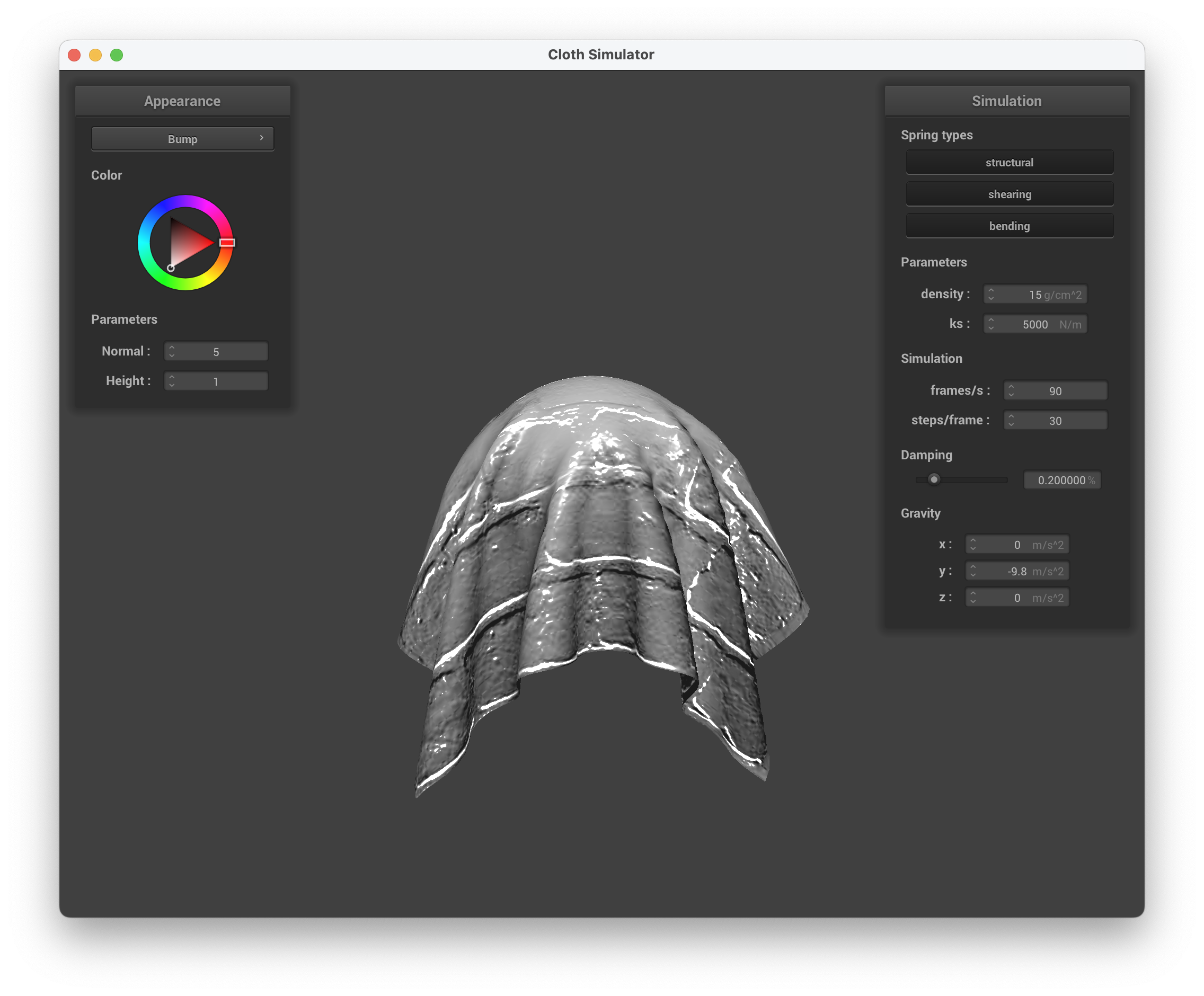
../scene/sphere.json, Bump Mapping
On the other hand, for displacement mapping, we are also adjusting the actual position of the vertices to match the map, creating the displacement that we see on the object. All together, we have the bump created by the new normals that we calculated, as well as varying vertex positions to account for corresponding displacements. We did this by updating Displacement.vert and changed gl_position since it represents the screen space position.
Below are screenshots of running ./clothsim -f ../scene/sphere.json with displacement mapping, setting the normal to 100 and height to 0.05, using texture3.png.
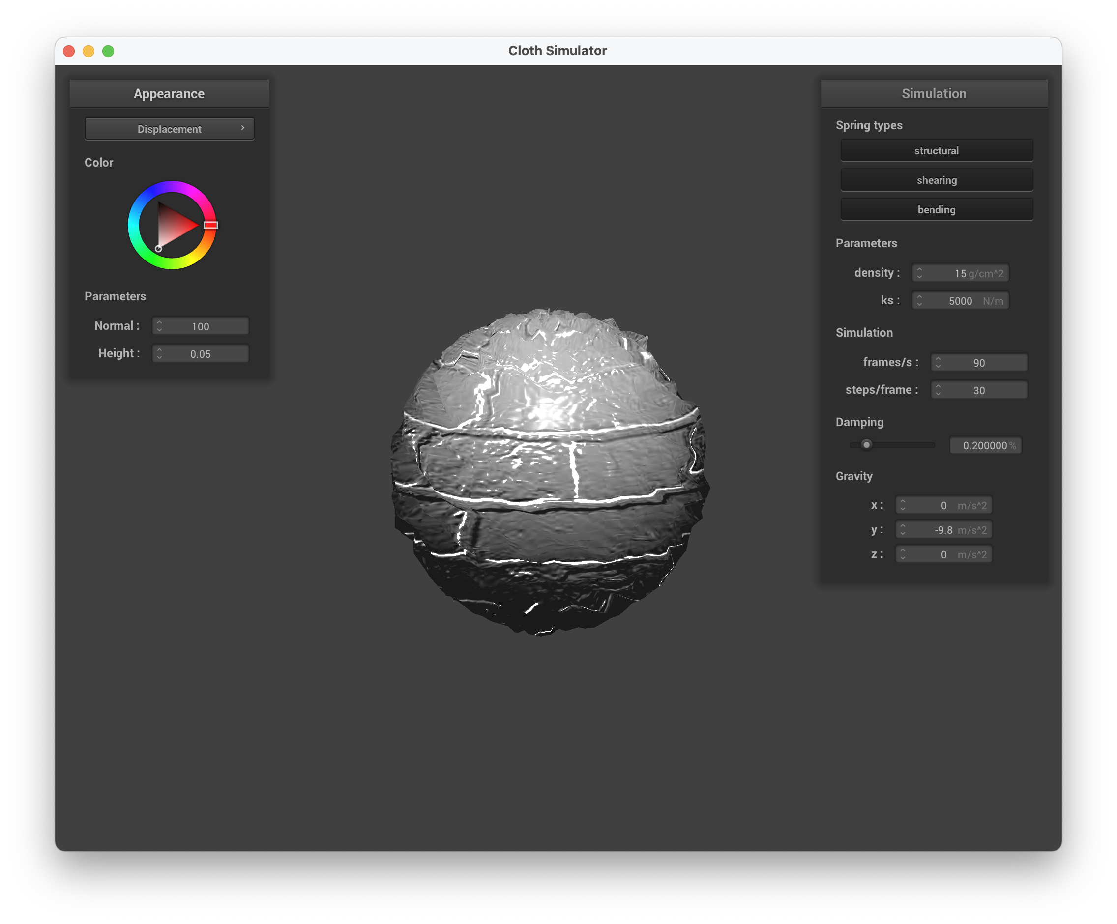
../scene/sphere.json, Displacement Mapping on the Sphere
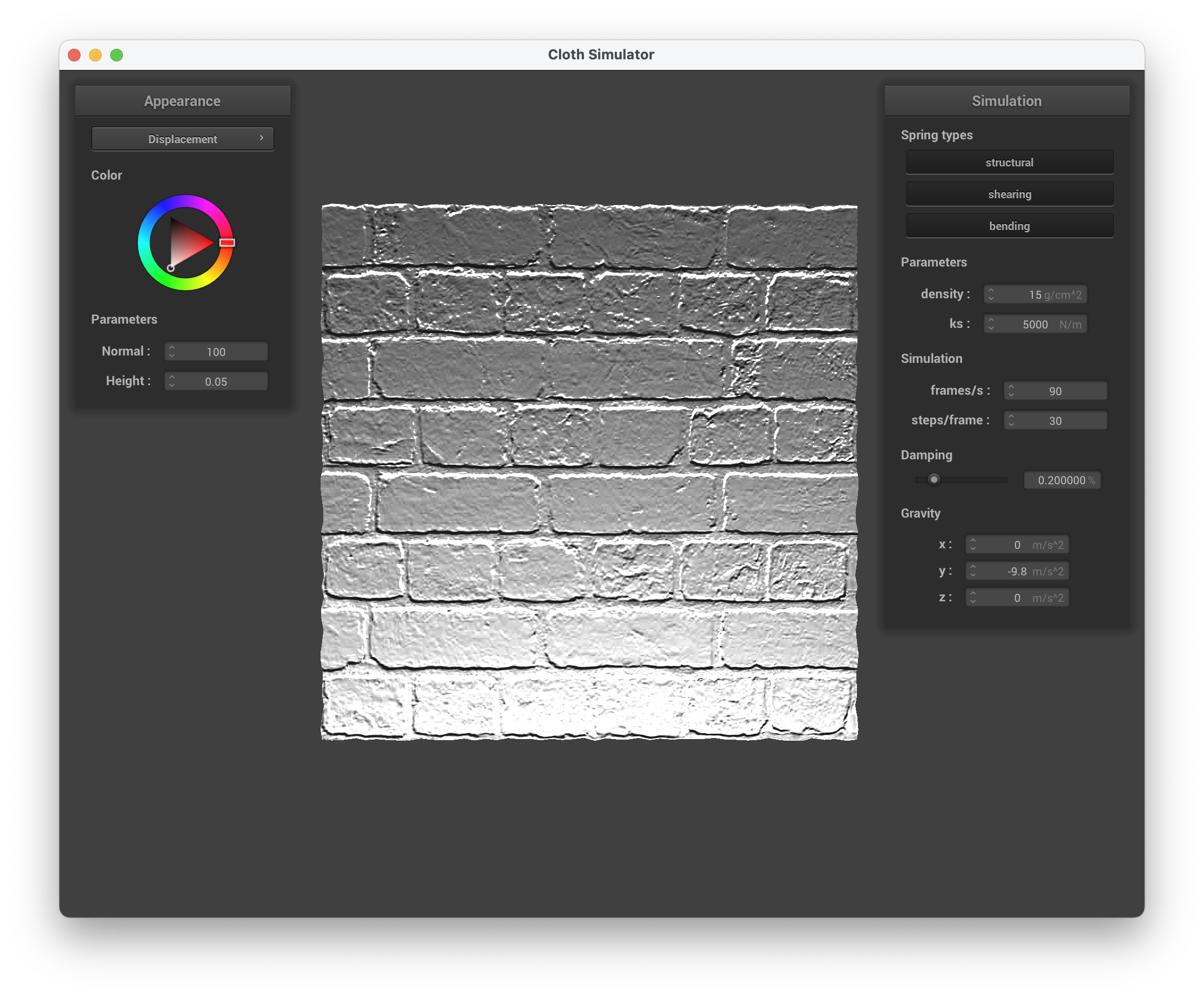
../scene/sphere.json, Displacement Mapping on the Cloth
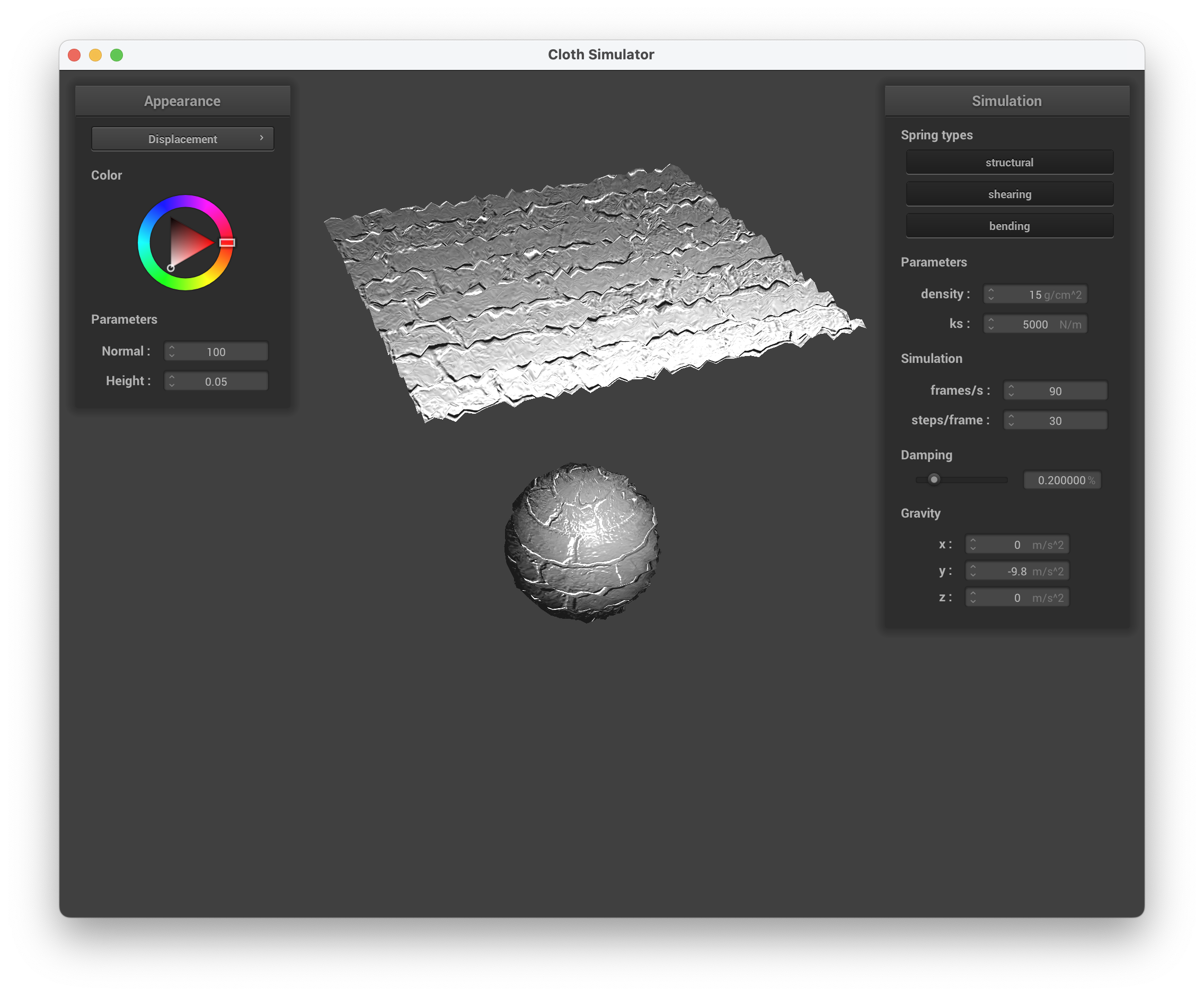
../scene/sphere.json, Displacement Mapping on the Sphere and Cloth
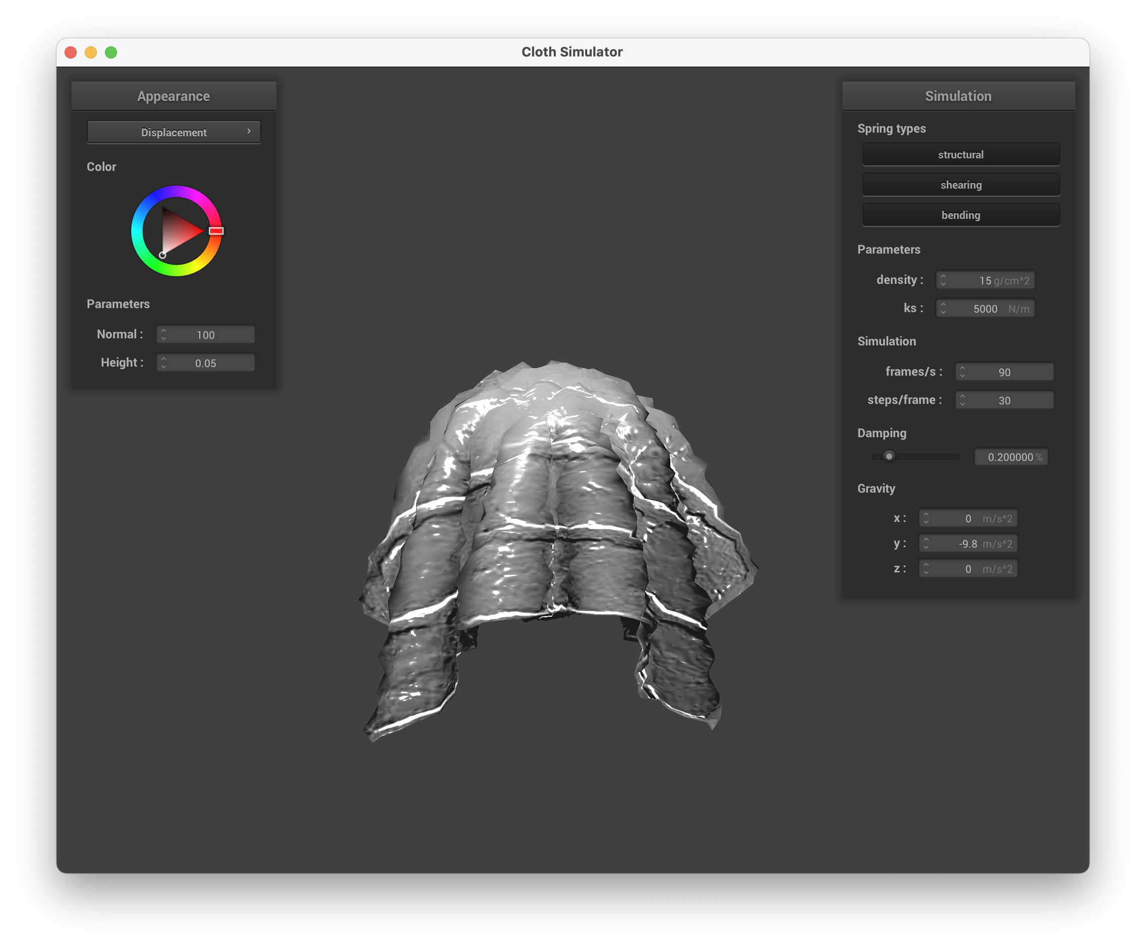
../scene/sphere.json, Displacement Mapping

../scene/sphere.json, Bump Mapping on the Sphere

../scene/sphere.json, Displacement Mapping on the Sphere

../scene/sphere.json, Bump Mapping on the Sphere and Cloth

../scene/sphere.json, Displacement Mapping on the Sphere and Cloth
We can see that bump mapping still maintains the smoothness of the sphere since only the fragments are modified, creating the visual effect of bumps and indents. On the other hand, displacement mapping changes the location of each vertex, causing it to be more deformed and "spiky".
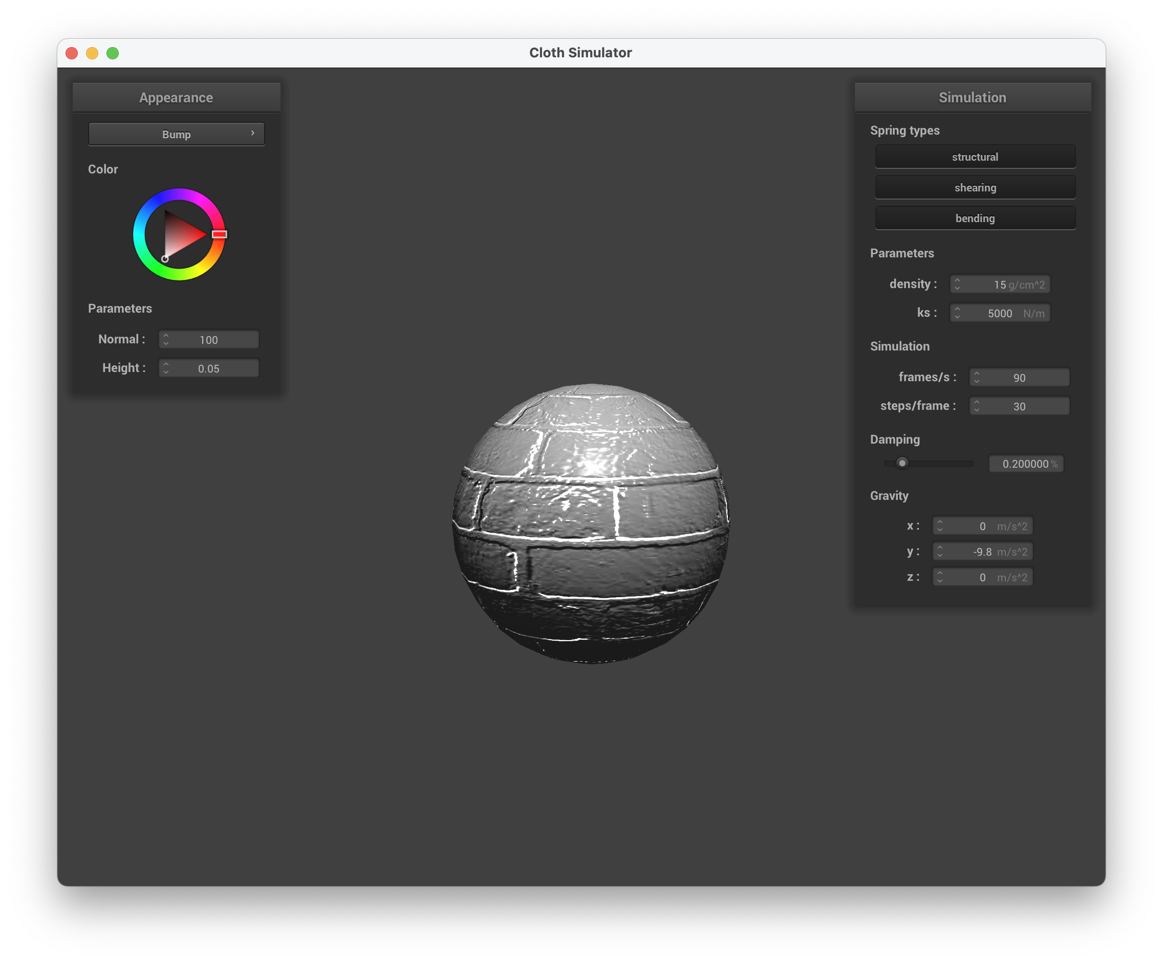
../scene/sphere.json, Bump Mapping -o 16 -a 16
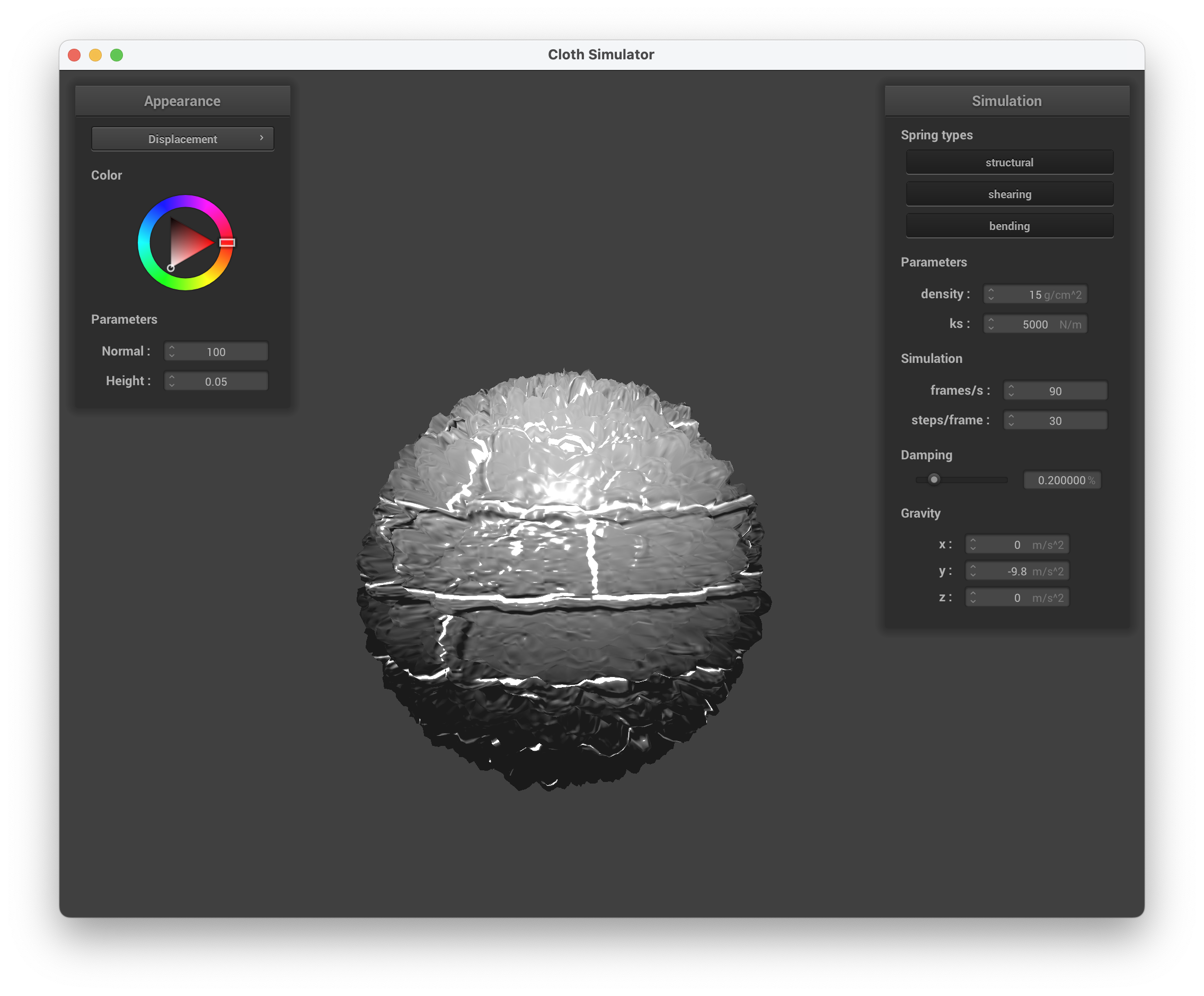
../scene/sphere.json, Displacement Mapping -o 16 -a 16
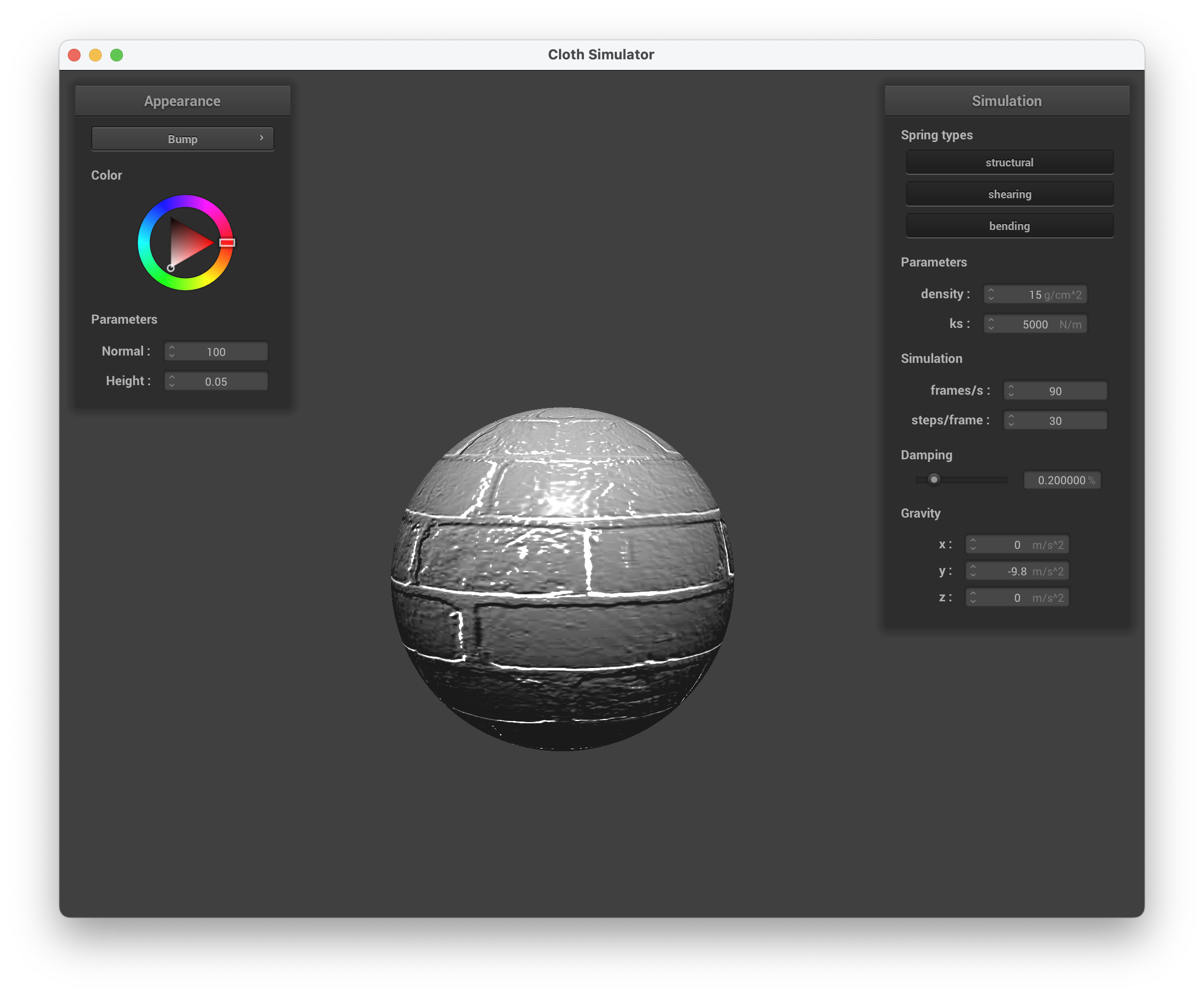
../scene/sphere.json, Bump Mapping -o 128 -a 128

../scene/sphere.json, Displacement Mapping -o 128 -a 128
Above are screenshots of running ./clothsim -f ../scene/sphere.json with bump and displacement mapping, setting the normal to 100 and height to 0.05, using texture3.png. The coarseness is altered by -o 16 -a 16 and -o 128 -a 128.
When changing the coarseness of the sphere, we can immediately see that displacement mapping impacts coarseness more than bump mapping does. With lower coarseness, there's less sampling points to change the vertices of, hence why there are jumps and the sphere appears more "spikey". At a higher resolution, the coarseness is higher and the surface texture of the sphere is more realistic. The spikes are also less pronounced because more vertices' positions are displaced, causing the overall sphere to apear more "round".
With bump mapping, there is little difference in the sphere's shape because the positions of the vertices don't change.
In this task, we want to create a shader that creates a direct reflection of the environment, like a mirror. We do this by finding the outgoing eye-ray, \(w_o\) by subtracting the camera's position u_cam_pos from the fragment's position (v_position). Then, we calculate the incoming eye-ray, \(w_i\) with the formula \(w_o - 2(w_o * n) * n\). Afterwards, we sample the texture for the incoming direction \(w_i\) calculated.
Show a screenshot of your mirror shader on the cloth and on the sphere.
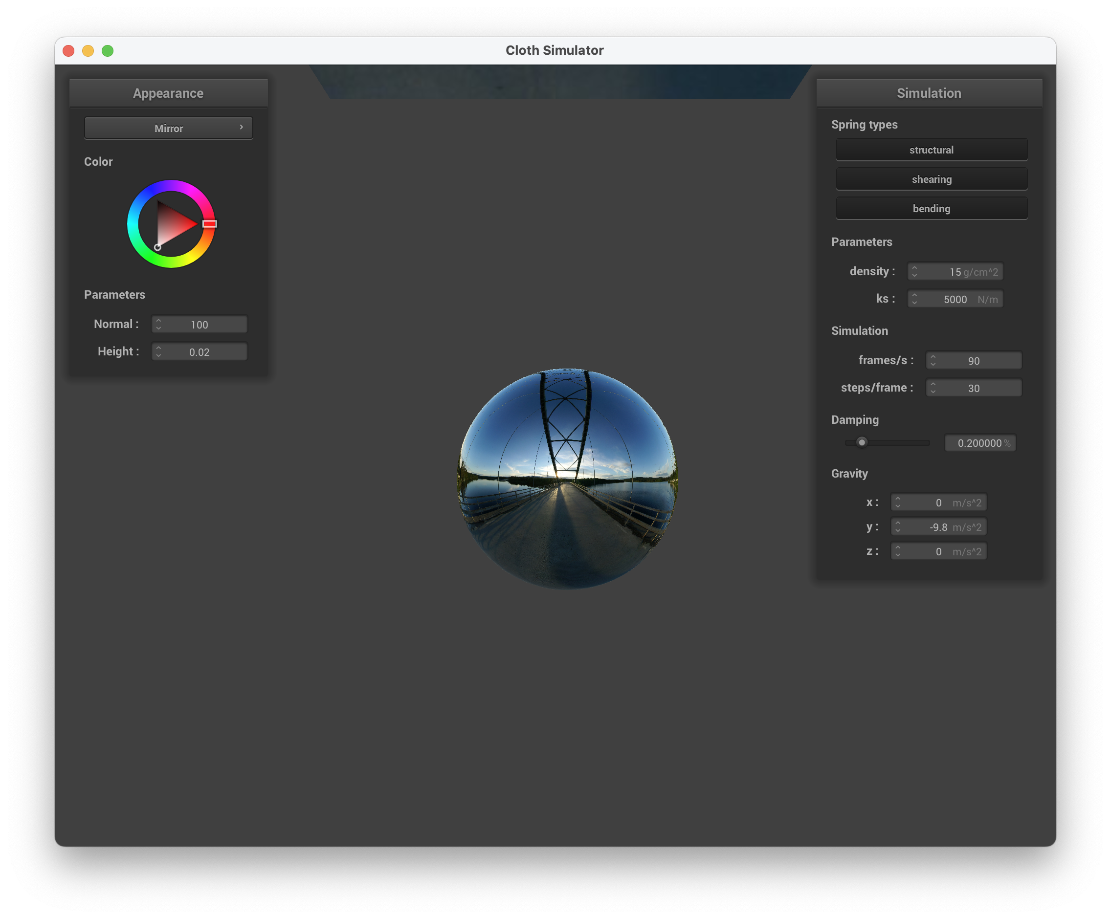
../scene/sphere.json, mirror shader on the sphere
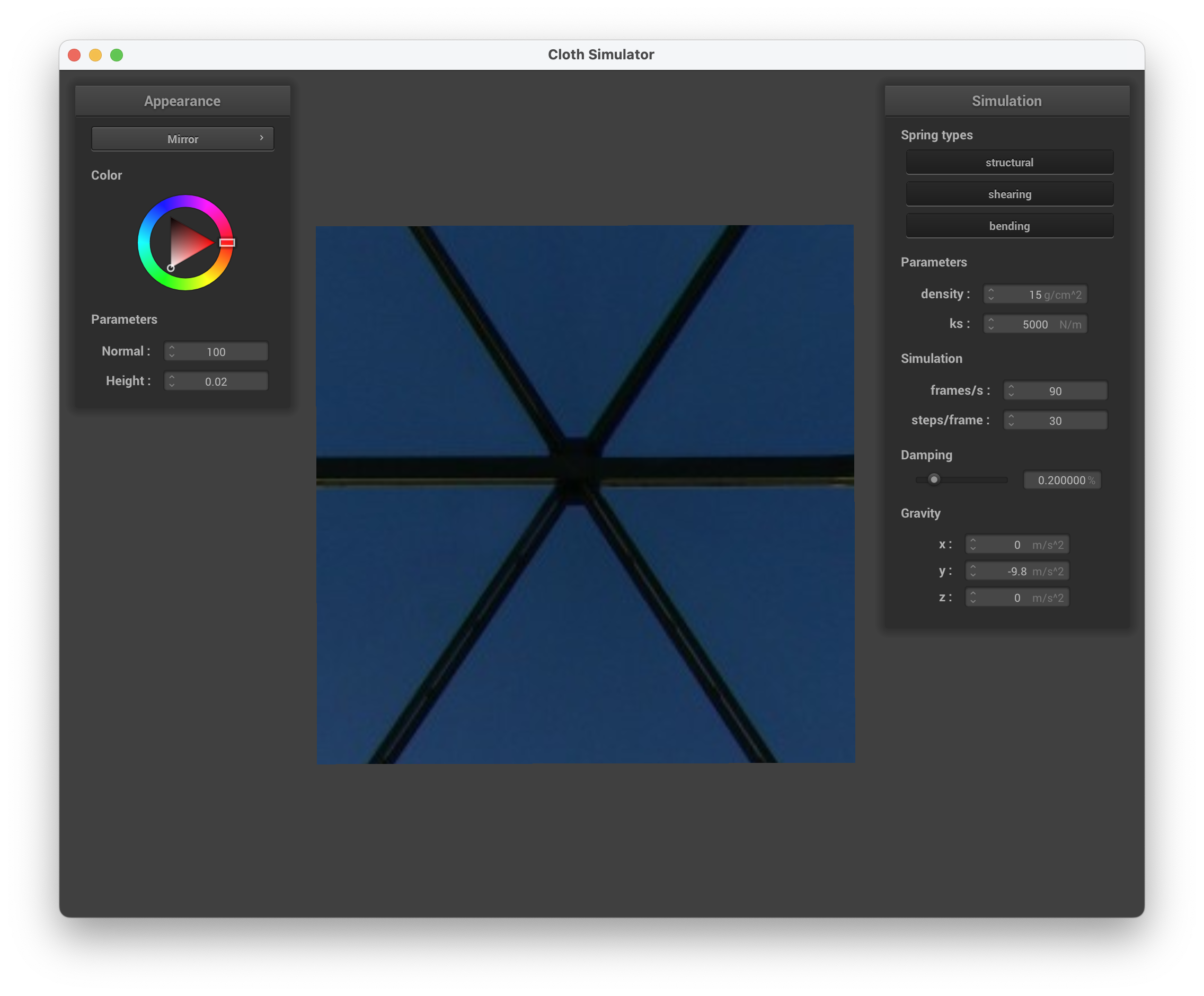
../scene/sphere.json, mirror shader on the cloth
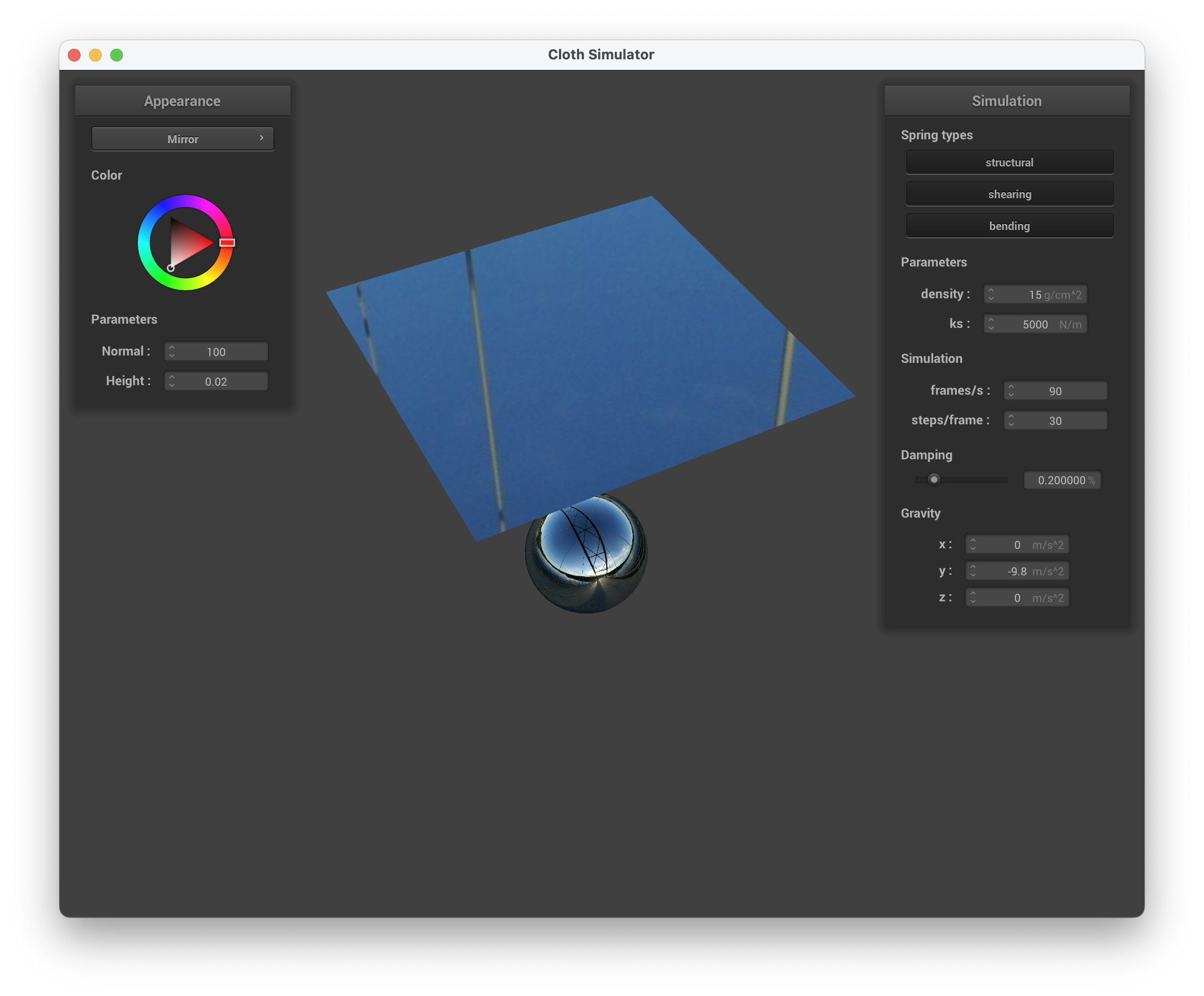
../scene/sphere.json, mirror shader on the sphere and cloth
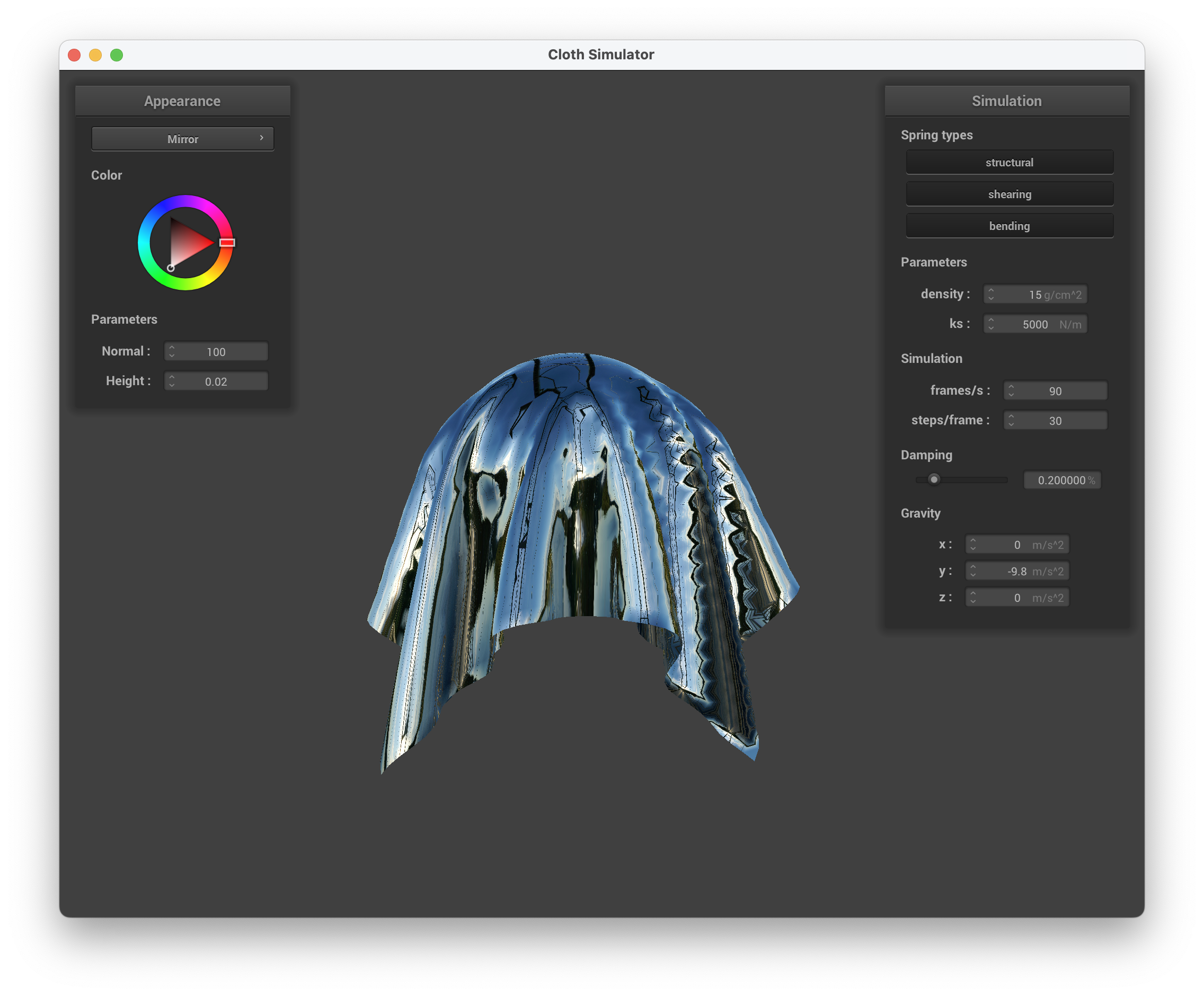
../scene/sphere.json, mirror shader
In preparation for our final project, we wanted to get experience with building our custom shader. We intended to simulate the appearance of water with random darker dots on the surface (i.e static on an old TV screen) and the final output is similar to that.
To generate the random dots, we initially searched for a random function in GLSL but couldn't find one. Therefore, we created our own random number generator based on this source and adjusted the numbers accordingly. The function returns a random number between 0 and 1.
If the random number is < 0.5, we set all the k_coefficients to 0.4. Otherwise, we set all the k_coefficients to 0.9. The shader calculates the dots by multiplying the normal vector v_normal.xyz with the coefficients. This adjusts the darkness of the dots based on the surface normal.
To create the blue color of water, we experiment with different RGB values and added that to our vector of dots. We attempted to create the transparent/translucence appearance of water via vec4 transparent_water = vec4(water_color, 0.5) which semi-worked. This was done by combining the water color with an alpha value, resulting in partial transparency.
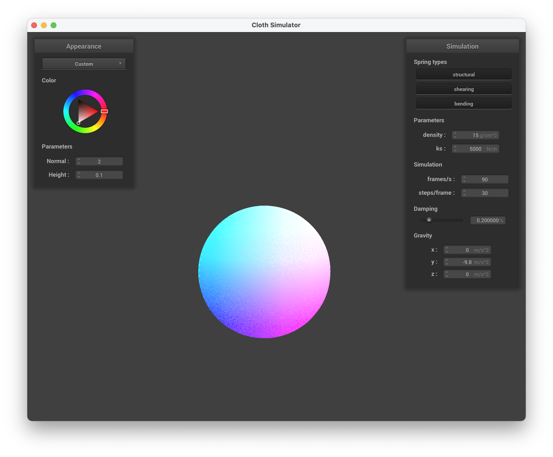
../scene/sphere.json, sphere view with custom shader
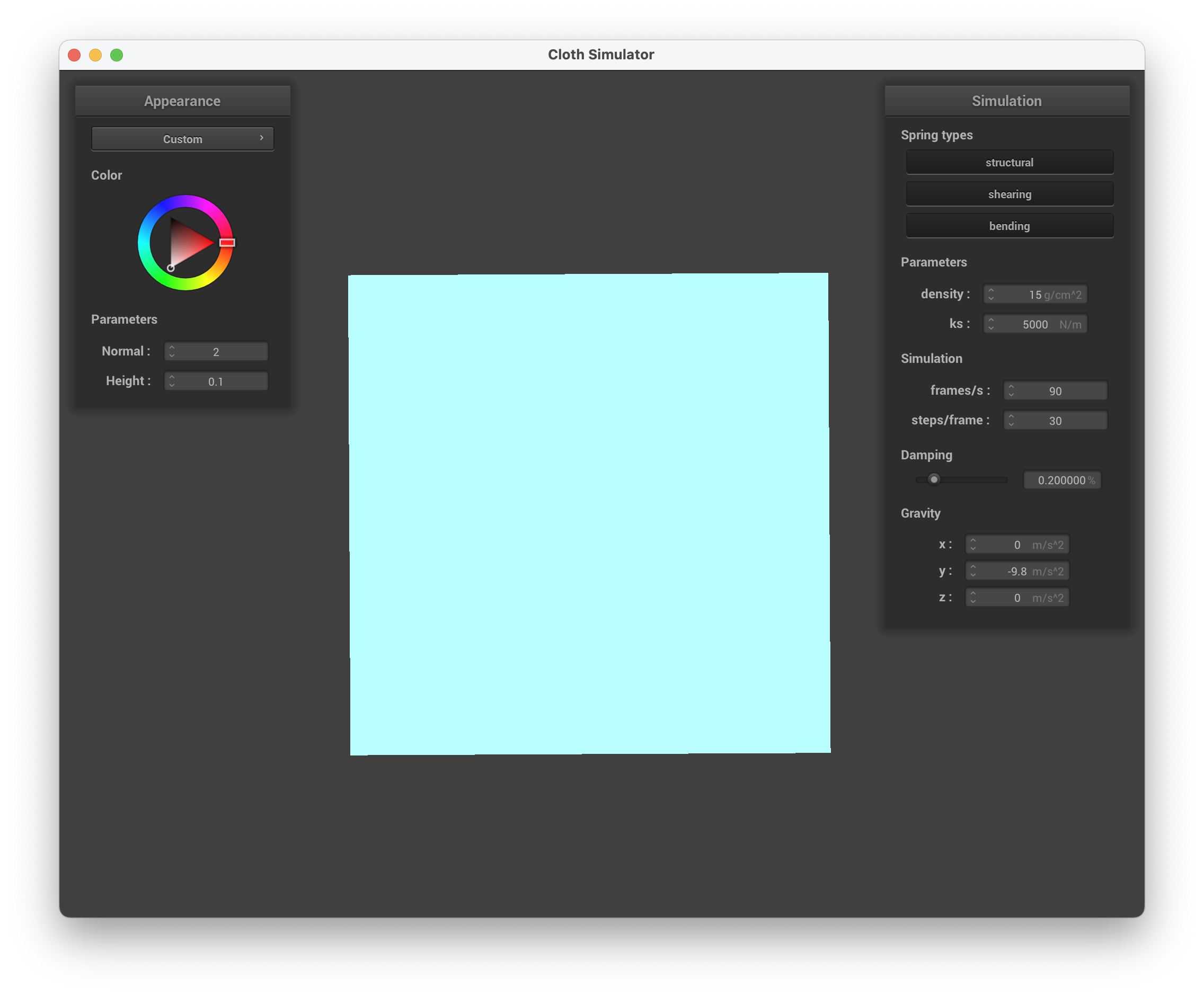
../scene/sphere.json, cloth view with custom shader
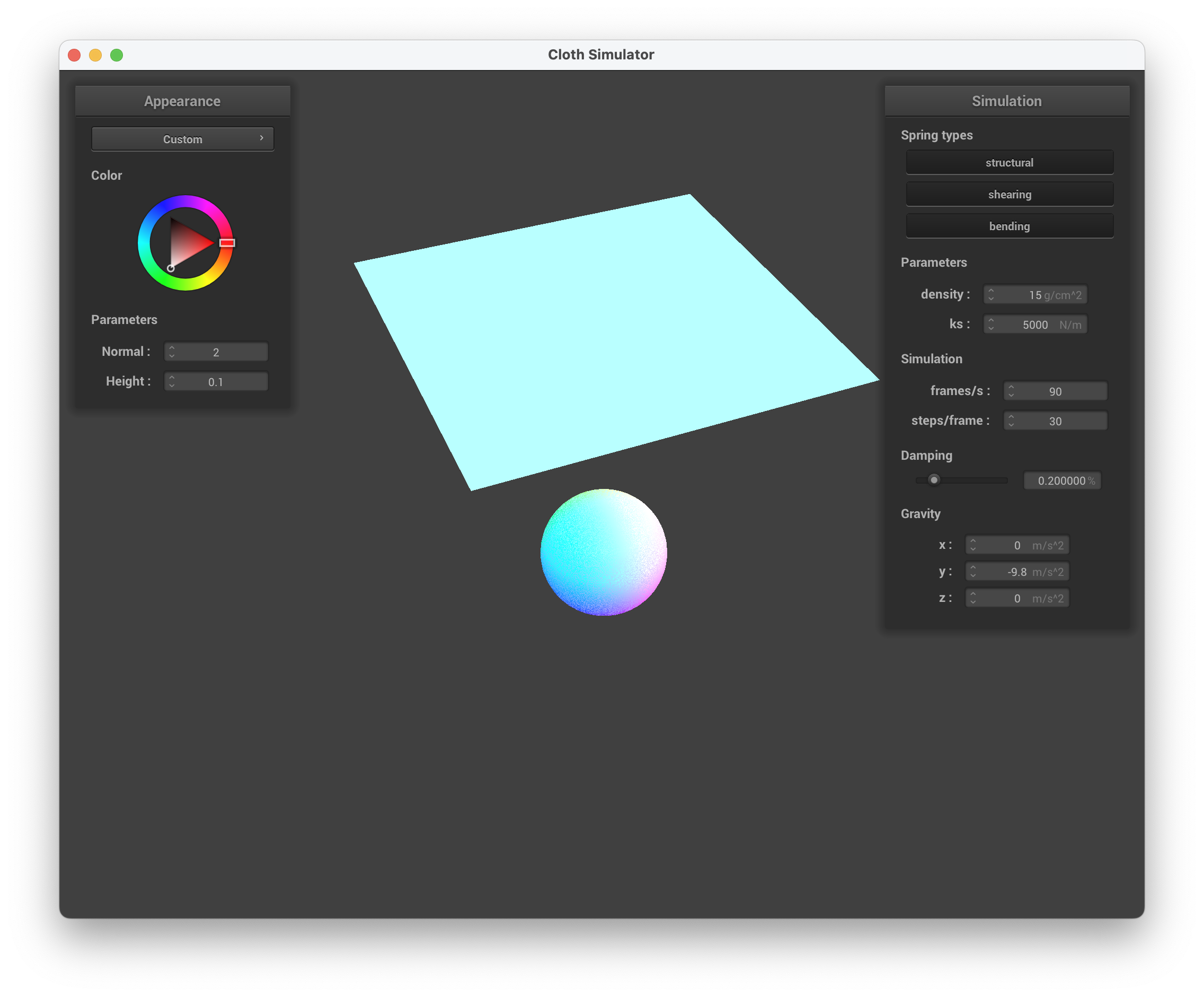
../scene/sphere.json, sphere and cloth view with custom shader
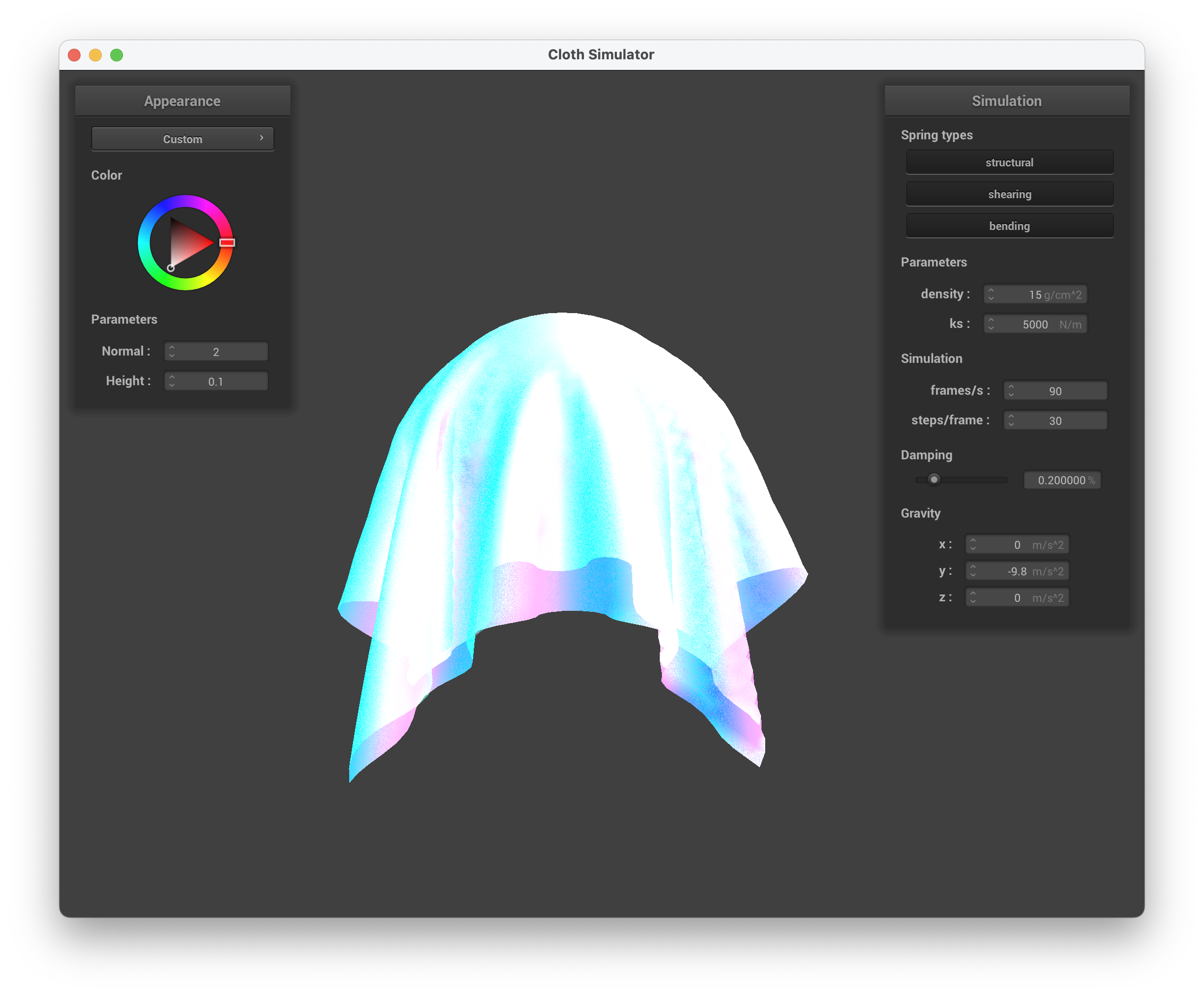
../scene/sphere.json, view with custom shader
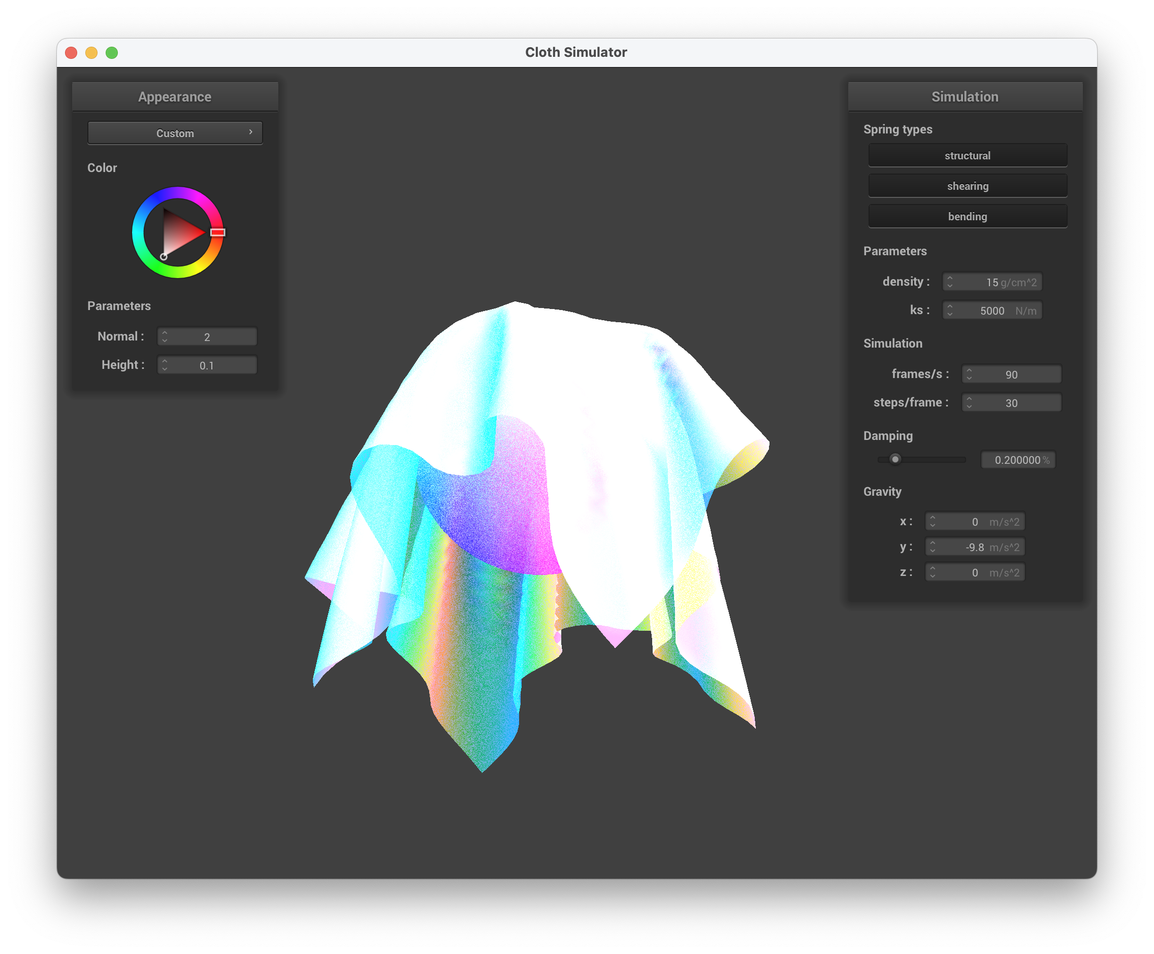
../scene/sphere.json, underneath the cloth with custom shader, showcasing the random dots
The shader is "holographic" on the underside of the cloth while the sphere is a combination of light blue, dark blue, pink, and white. The top of the cloth is more translucent, where the screenshot of the cloth on the sphere gives off the illusion of the ball not being present. Overall, the shader mimics a glossy and thin sheet of holographic paper on the underside, while resembling a shiny jellyfish body from the side view to me.