Website URL: Here

I hate CBbunny.dae
Overview
The purpose of this homework is to learn how to implement the different components of a ray tracer. First, we learned how to convert between camera space and world space, allowing us to generate samples and intersect rays with triangles and spheres with the Möller-Trumbore algorithm. We were able to construct a BVH to accelerate ray tracing. Splitting points are chosen based on a heuristic and we split primitives into BVH nodes.
Direct illumination was the next component we learned to implement, consisting of uniform hemisphere sampling and importance sampling. This allowed us to see the difference between the two sampling methods. Global illumination is a combination of indirect and direct lighting, which we incorporated next. Within global illumination, multi-bounce rendering and Russian Roulette rendering were aspects included to demonstrate their impact on the image result and rendering speed. Lastly, adaptive sampling gave us the ability to optimize rendering efficiency - specifically calculating to sample more on "difficult" locations versus sampling less on locations where pixels converged faster.
Ultimately, this project was extremely difficult since we faced many bugs during the peak of midterm season, but we were able to implement various ray tracing techniques and render cool images!
Part 1: Ray Generation and Scene Intersection
Task 1: Generating Camera Rays
When generating camera rays, we need to transform the image coordinates (x, y) to camera space by interpolation. In the camera space, the camera is positioned at (0, 0, 0) and looks along its -Z axis. There is an axis-aligned rectangular virtual camera sensor that lies on the Z = -1 plane which is why we need to use hFov and vFov field of view angles along the `X and Y axis to transform into camera space. For normalized image coordinates, (0, 0) is the camera origin so we needed to first shift the normalized x and y coordinates to align the Z axis and rescale the normalized coordinates.
Now, in 3-dimensional camera coordinations, we have the vector direction containing x, y, and -1. This is the ray direction vector which is used to transform the camera space ray to world space using the camera-to-world rotation matrix, c2w (a 4x4 homogeneous coordinate system transform matrix). Afterwards, we need to normalize d. For the defined ray, the camera is placed at pos (camera position in world space) which is utilized as column 4 and to set the range for the clipping planes, we initialized min_t and max_t of the Ray with nclip and fclip respectively.
Task 2: Generating Pixel Samples
After creating the camera rays in world space, we generate pixel samples by first generating ns_aa random samples within the pixel. While iterating through all of the pixel samples, we obtain a random sample and normalize the coordinates. Then, we call camera->generate_ray, passing in the normalized (x, y) coordinates, and then call est_radiance_global_illumination to estimate the radiance. After all the samples are processed, we averaged out the pixel color with vec_sum = vec_sum/num_samples and update the sampleBuffer by calling update_pixel with that color.
Task 3: Ray-Triangle Intersection
To implement ray-triangle intersection, we used Möller-Trumbore intersection algorithm derived from lecture. The Triangle::has_intersection method allows us to test whether there is an intersection between a triangle and the input ray. The bulk of this algorithm lies within the intersection algorithm used where these parameters are computed using the Möller–Trumbore algorithm and determine if and where the ray intersects with the plane of the triangle, and then checks if the intersection point lies within the triangle itself.
-
test_vec.xcontains the parametertof the ray equation where the intersection occurs -
test_vec.ycontains the parameterb1, which represents the barycentric coordinate of the intersection point with respect to the triangle's vertices -
test_vec.zcontains the parameterb2, another barycentric coordinate
Intersection Testing:
-
If any of the barycentric coordinates
(b1, b2)are less than0or their sum is greater than1, it means the intersection point lies outside the triangle so the function returns false -
If the parameter
tis outside the valid range[r.min_t, r.max_t], the intersection point is not within the segment of the ray being considered so the function returns false -
Otherwise,
r.max_tis updated totto limit the maximum intersection distance of the ray and returns true, indicating an intersection has been found
If an intersection is found, the function updates the intersection data (isect) with relevant information:
-
t: the parametertof the ray equation where the intersection occurs -
n: the surface normal at the intersection point calculated as the weighted sum of the triangle's vertex normals (n1,n2,n3) based on the barycentric coordinates -
primitive: a pointer to the triangle primitive that was intersected -
bsdf: a pointer to the surface material (BSDF) at the hit point
Essentially, we combine Barycentric coordinates and an implicit definition of a plane to determine whether the intersection point resides inside a triangle primitive.
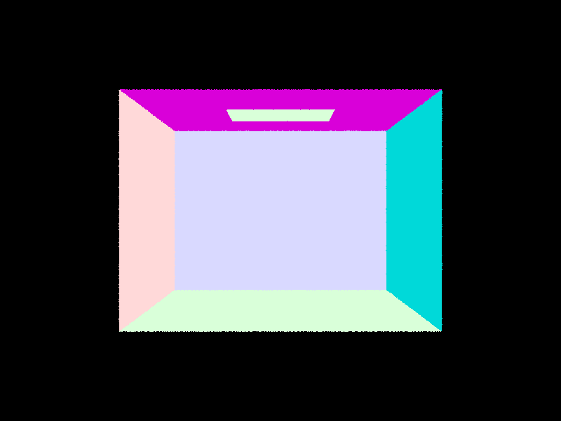
Screenshot of CBempty.dae
Task 4: Ray-Sphere Intersection
Ray-sphere intersection was similar since it incorporates the Möller-Trumbore intersection algorithm but a bit more involved than ray-triangle intersection. There is a new test method which returns true if there are intersections and writes the smaller of the two intersection times in t1 and the larger in t2. Within these methods, we reduce the intersection points to the roots of a quadratic equation and the discriminant is used to determine the number of intersections.
-
a: represents the squared magnitude of the ray direction (r.d) -
b: represents the dot product between the ray direction and the vector from the ray origin to the sphere center -
c: represents the squared magnitude of the vector from the ray origin to the sphere center minus the squared radius of the sphere -
t_plus,t_minus: variables to store the potential intersection times calculated using the quadratic formula
As such, if discriminant is less than 0, this means that the ray missed the sphere/doesn't intersection so we return false. If discriminant is non-negative, this indicates that there is at least one real root so we used the quadratic formula to determine the time of intersection and assign t_plus and t_minus. The function compares t_plus and t_minus to determine which one is smaller and larger in order to assign the smaller intersection time to t1 and the larger one to t2.
If an intersection is found within the valid range [r.min_t, r.max_t] and t1 is adequately updated using the test helper method, has_intersection updates r.max_t to the intersection time t1 (the smaller of the two intersection times) and returns true. In intersection, we do the same in addition to populating i (Intersection object) as stated in the spec (t, primitive, bsdf) and the surface normal.
Here are some images with normal shading for a ew small .dae files:
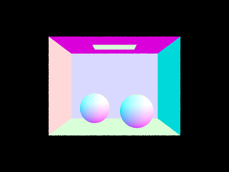
../dae/sky/CBspheres_lambertian.dae
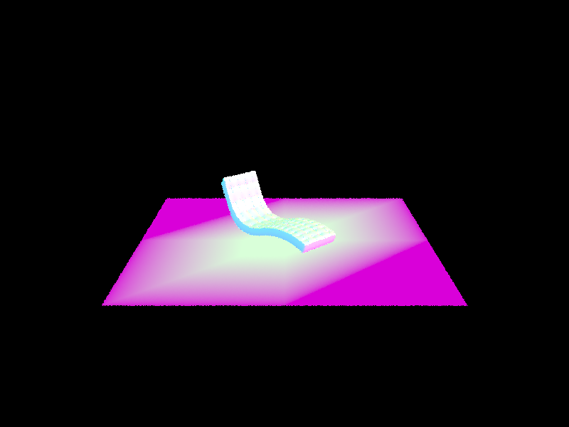
../dae/sky/bench.dae
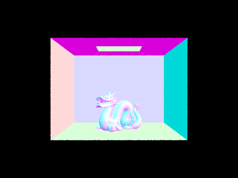
../dae/sky/CBdragon.dae
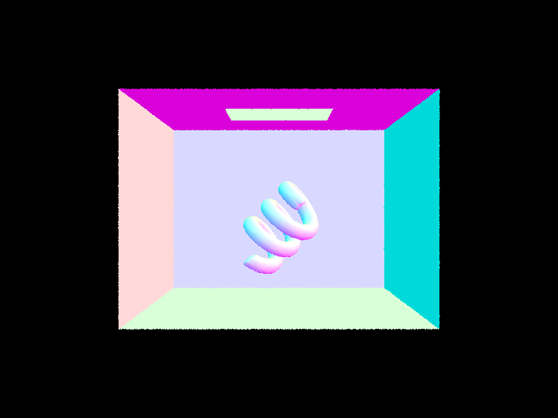
../dae/sky/CBcoil.dae
Part 2: Bounding Volume Hierarchy
Task 1: Constructing the BVH
In BVHAccel::construct_bvh, we first generate the outermost bounding box that encloses all the primitives in the given range (start to end). We iterate through all the primitives passed in the range and expand the bounding box to include each primitive's bounding box.
We create a new BVHNode if the number of primitives (num_prim) is less than or equal to the max_leaf_size and initialize its start and end to be the start and end of the primitives.
If not, we need to recurse and determine the split point and axis selection to split up the bounding volume hierarchy. First, we computed the average centroid across all the primitives' bounding boxes within the node. This centroid is used to determine the split axis for partitioning the primitives. The split axis is chosen as the axis that results in the smallest bounding box heuristic among the three axes (X, Y, Z). The bounding box heuristic is calculated based on the surface area of the child bounding boxes after splitting and the primitives are partitioned into left and right child nodes based on the chosen split axis and the average centroid.
We chose to use the mean position as the split point instead of the median because we would have to sort the primitives along each axis first. Adding the sort step in the recursion increases the time for generating the BVH. Additionally, a general ray-tracer should work well without prior information about the 3D distribution of primitives so we can assume that for an arbitrary scene, the probability of finding a primitive at any point 3D space follows a uniform distribution so the mean centroild location and median centroid location across the axes are approximately equal.
left_primitives and right_primitives are used to store primitives on the left and right sides of the split axis which are then redistributed into the left and right vectors based on their centroid positions along the split axis. Within the loop, if the index i is less than the size of the left_primitives vector, it means there are still primitives left to be assigned to the left child node. If i exceeds the size of the left_primitives vector, it means all left primitives have been assigned, and the remaining primitives need to be assigned to the right child node.
Recursive calls to construct_bvh are made to construct the left and right child nodes. For the left child node, the range of primitives is from start to the iterator center_left and for the right child node, the range is from center_left to end.
The images below show how utilizing a 3-axis heuristic is better than splitting along only the mean x-coordinate. The bounding boxes encapsulate the primitives more tightly which reduces the probability that a ray hits the bounding box of a BVH without hitting a primitive.
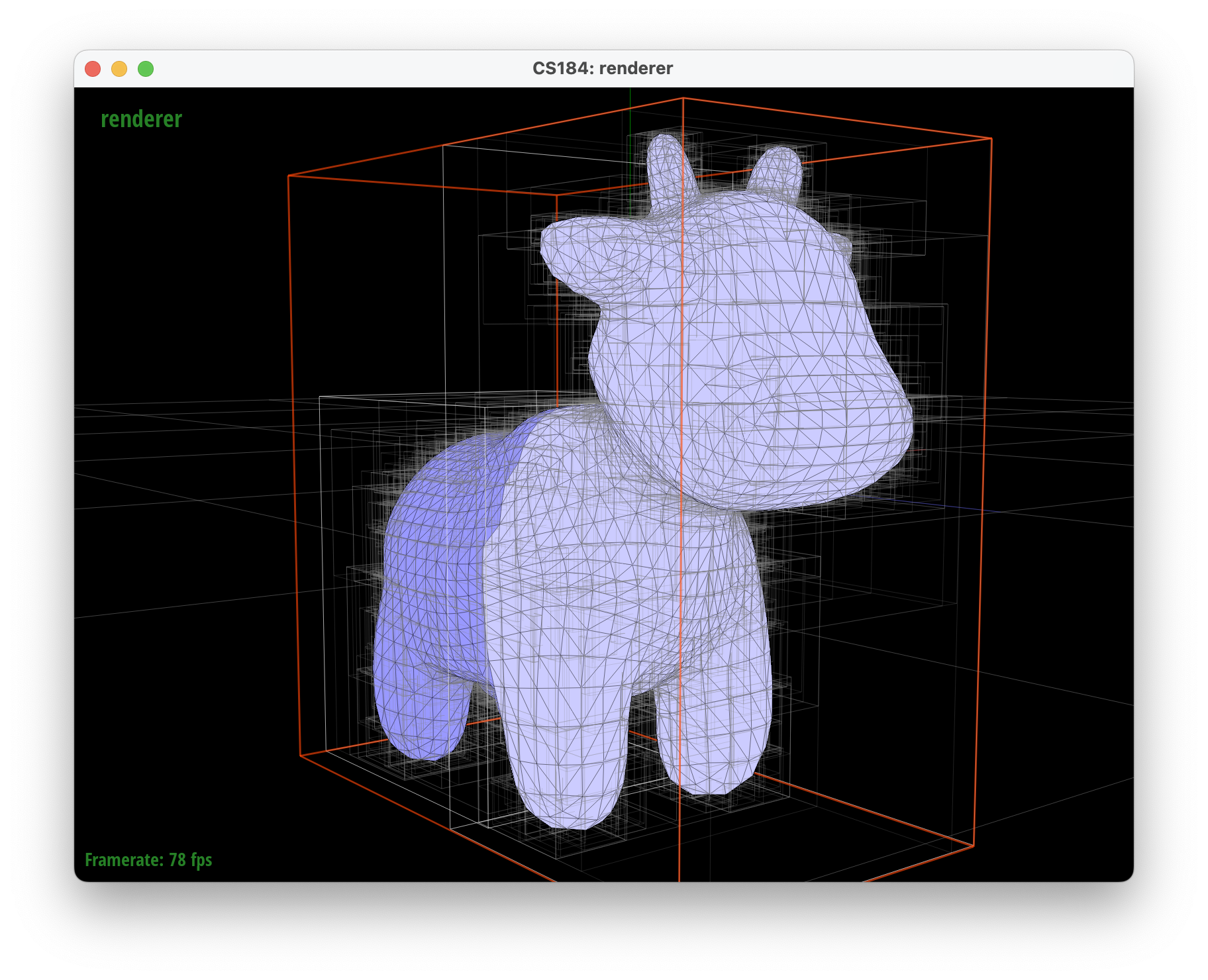
../dae/meshedit/cow.dae, base rendering
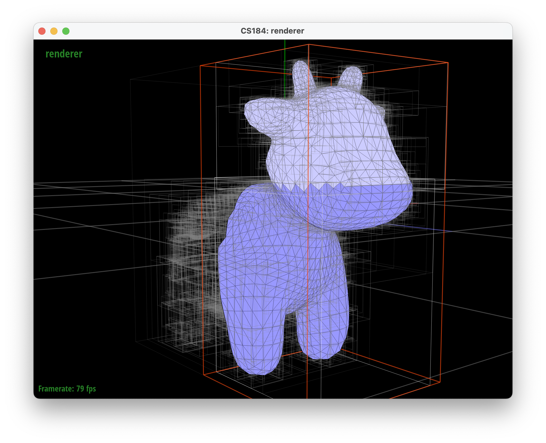
../dae/meshedit/cow.dae, descending once to right child
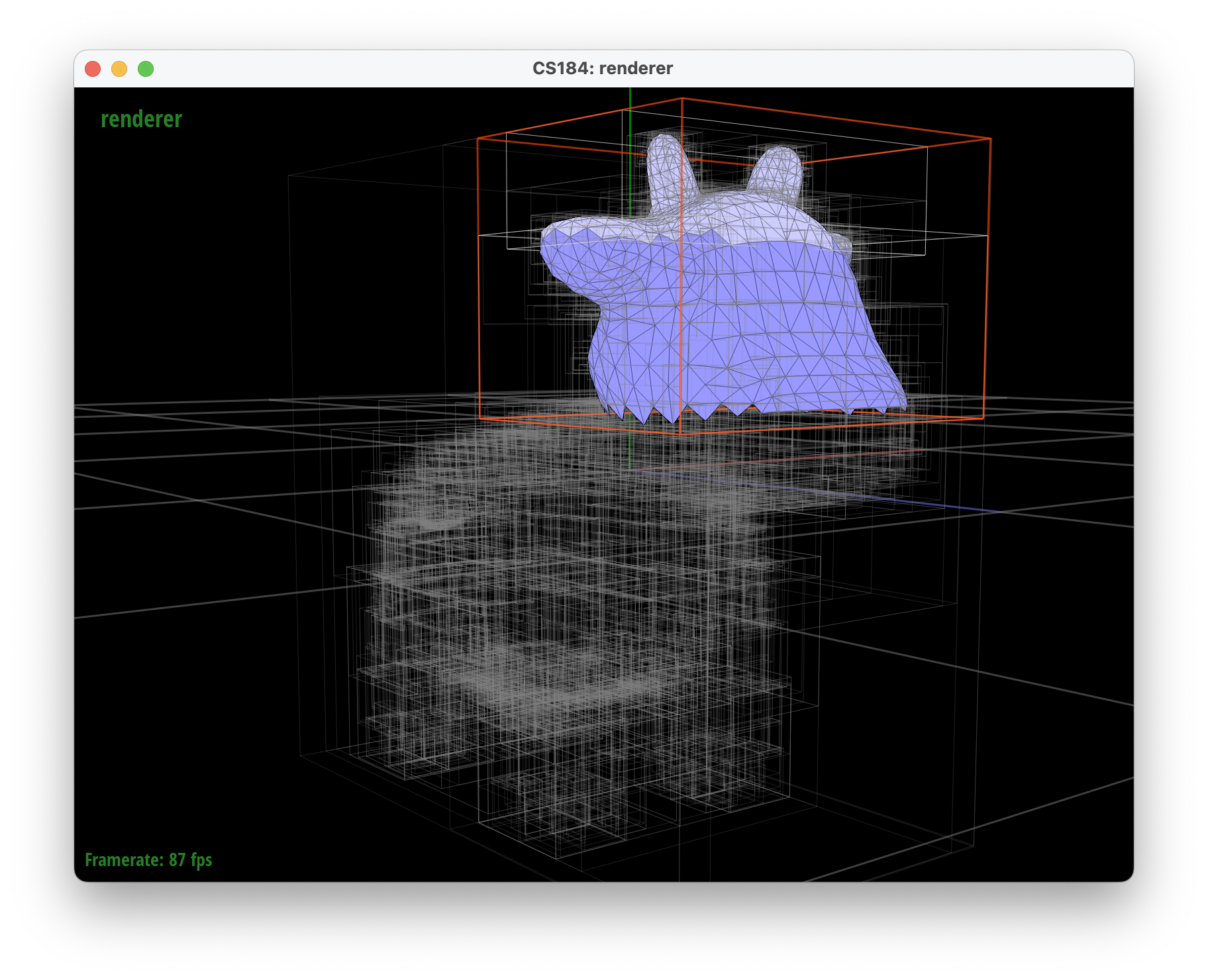
../dae/meshedit/cow.dae descending twice
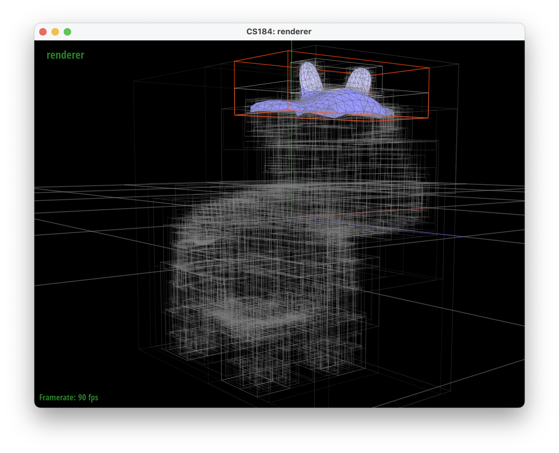
../dae/meshedit/cow.dae descending three times
Task 2: Intersecting the Bounding Box
Implementing BBox::intersect utilizes the given ray and axis-aligned plane intersection and ray and axis-aligned box intersection equations to check whether a ray intersects a given bounding box.
Time is represented as \( t = \frac{{p_x' - o_x}}{{d_x}} \) when perpendicular to the x axis. Intersection times (t) are calculated for each axis using the parametric equation of a ray, where \( t = \frac{{p[\text{axis}] - o[\text{axis}]}}{{d[\text{axis}]}} \). This equation represents the intersection of the ray with each of the bounding box's six planes along the X, Y, and Z axes. The minimum and maximum intersection times (min_t and max_t) are calculated for each axis which represent the entry and exit points of the ray into and out of the bounding box along each axis. Specifically, the interval of intersection is determined by taking the maximum of the minimum intersection times (min_t) across all axes and the minimum of the maximum intersection times (max_t) across all axes, ensuring that the intersection interval is as tight as possible.
If the max of min_t is greater than the min of max_t, it indicates that the ray misses the bounding box along at least one axis which is why we return false (no intersection). Otherwise, t0 and t1 are updated directly if an intersection is found within the provided range and we return true.
Task 3: Intersecting the BVH
The following times were collected by calling ./pathtracer -t 8 -r 800 600 -f {filename}.png ../dae/{path to file}.dae with and without BVH acceleration.
| File | Without BVH Acceleration | With BVH Acceleration |
|---|---|---|
../dae/sky/dragon.dae |
114.1280 seconds | 0.027 seconds |
../dae/sky/CBbunny.dae |
31.9542 seconds | 0.0211 seconds |
../dae/sky/CBlucy.dae |
50.7390 seconds | 0.0490 seconds |
../dae/meshedit/maxplanck.dae |
144.7978 seconds | 0.0375 seconds |
| File | Intersection Tests Per Ray (Without BVH) | Intersection Tests Per Ray (With BVH) |
|---|---|---|
../dae/sky/dragon.dae |
26331.172812 tests per ray | 13.020385 tests per ray |
../dae/sky/CBbunny.dae |
5180.986541 tests per ray | 14.620026 tests per ray |
../dae/sky/CBlucy.dae |
67920.405738 tests per ray | 10.578069 tests per ray |
../dae/meshedit/maxplanck.dae |
9767.330203 tests per ray | 13.643585 tests per ray |
With BVH acceleration, the computational efficiency is significant. For example, the ../dae/sky/dragon.dae rendering completed after 0.027 seconds with BVH acceleration while it took 114.1280 seconds without BVH acceleration. Resepectively, there were 26331.172812 intersection tests per ray without BVH acceleration and 13.020385 intersection tests per ray with BVH aceleration showcasing how without using BVH acceleration, the average number of intersection tests per ray is O(n) and with BVH acceleration is O(log n) where n is the number of primitives in the scene.
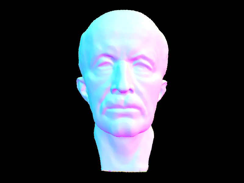
../dae/meshedit/maxplanck.dae after BVH acceleration
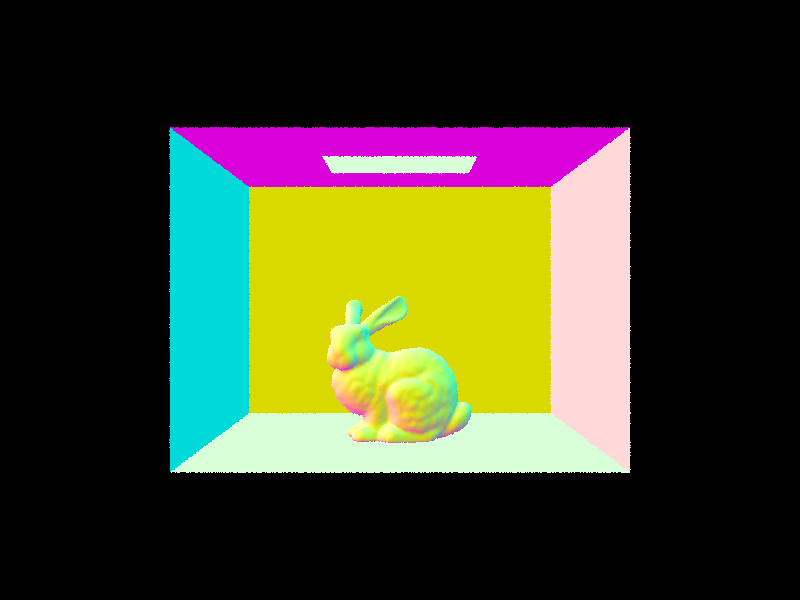
../dae/sky/CBbunny.dae after BVH acceleration
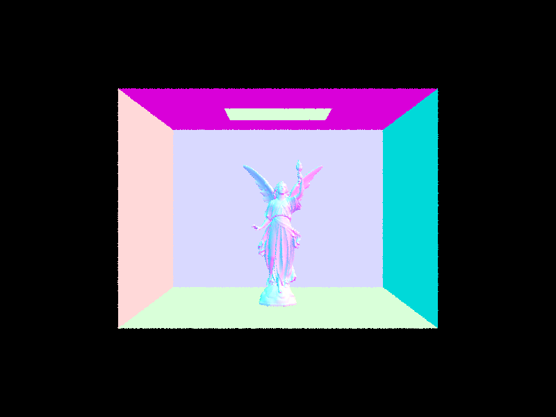
../dae/sky/CBlucy.dae after BVH acceleration
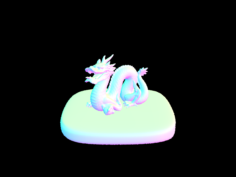
../dae/sky/dragon.dae after BVH acceleration
Part 3: Direct Illumination
Task 1: Diffuse BSDF
DiffuseBSDF::f represents a diffuse material that reflects incoming light equally in all directions on the hemisphere. Originally, we returned the reflectance of the DiffuseBSDF but this didn't match the image in spec. The surface area of a unit hemisphere is \(2 \times \pi\) and based off of lecture slides, the integral of cosine over hemisphere is only 1/2 the area of the hemisphere, thus why we chose to divide reflectance by \( \pi \) and resulted in the correct matching image.
Task 2: Zero-bounce Illumination
To implement zero-bounce illumination, we obtained the Intersection object's bsdf attribute and called get_emission() to get the emission value of the surface material (light that results from zero bounces of light). Afterwards, we updated est_radiance_global_illumination to utilize this method and generate the following image when running ./pathtracer -t 8 -s 16 -l 8 -m 6 -H -f CBbunny_16_8.png -r 480 360 ../dae/sky/CBbunny.dae.
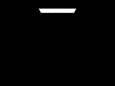
../dae/sky/CBbunny.dae with zero-bounce illumination
Task 3: Direct Lighting with Uniform Hemisphere Shading
With uniform hemisphere shading, we first iterated through num_samples samples by sampling a new_sample vector from the hemisphere after using hemisphereSampler. We calculated its world-space coordinates by multiplying it with o2w and created a new sample Ray (new_ray) with the new origin and direction. We made sure to also set new_ray's min_t to EPS_F.
Afterwards, we created a new Intersection labeled new_isect and checked whether the bounding volume hierarchy intersected the sampled Ray by calling intersect — the output returned was stored in a Boolean variable named is_intersected.
If there was an intersection, we calculated the L_i, f_r, \( \cos(\theta_j) \), and pdf values within the reflection equation to get the outgoing lighting. For L_i, this was simply obtaining the emission of the intersection's BSDF. To obtain f_r (f_result), we used the function we wrote in Task 1 to calculate the BSDF. Earlier, we calculated \( \cos(\theta_j) \) by finding the dot product between the surface normal of the intersection and the world-space unis of the ray. The pdf is the probability of sampling any point uniformly which is \( \frac{1}{{2 \pi}} \).
We created final_sample, which essentially helped us add \( \frac{{L_i \times f_r \times \cos(\theta_j)}}{{\text{pdf}}} \) to \( L_{\text{out}} \) for each sample Ray. After all iterations, we normalized L_out by dividing by num_samples.
Below are images of running ./pathtracer -t 8 -s 16 -l 8 -H -f CBbunny_H_16_8.png -r 480 360 ../dae/sky/CBbunny.dae, ./pathtracer -t 8 -s 64 -l 32 -m 6 -H -f CBbunny_H_64_32.png -r 480 360 ../dae/sky/CBbunny.dae and ./pathtracer -t 8 -s 64 -l 32 -m 6 -H -f CBempty.png -r 480 360 ../dae/sky/CBspheres_lambertian.dae with uniform hemisphere sampling.
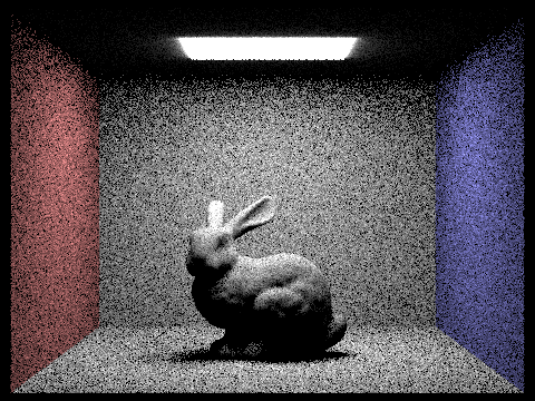
../dae/sky/CBbunny.dae 16 camera rays per pixel, 8 samples per pixel, uniform hemisphere sampling
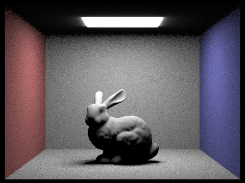
../dae/sky/CBbunny.dae 64 camera rays per pixel, 32 samples per pixel, uniform hemisphere sampling
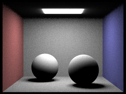
../dae/sky/CBspheres_lambertian.dae
Task 4: Direct Lighting by Importance Sampling Lights
Importance sampling is similar to uniform hemisphere sampling with the exception of now iterating through all the lights via scene->lights.begin(). First, we need to check whether is_delta_light() returns true if the light is a point light source. This is because if we sample a point light source, the ray's direction doesn't matter since the outgoing light is the same, hence why only one sample is needed. Otherwise, num_samples is equal to ns_area_light.
While still iterating through the lights, we now need to iterate through all of the samples for that light. We created a new vector L assigned to the output of calling sample_L, which also sets wi, distToLight and pdf. Following the same steps in uniform hemisphere sampling, we generated a new sample Ray (new_ray) and set it's min_T and max_T values to EPS_F and dist - EPS_F respectively. Afterwards, we created a new Intersection and checked if there was an intersection by using intersect.
If there isn't an intersection, we calculated the \( f_r \) to compute the reflection equation to get the outgoing lighting. This is because if there was an intersection, we don't want to illuminate it because of the previous intersection. We added \( \frac{{L_i \times f_r \times \cos(\theta_j)}}{{\text{pdf}}} \) to \( L_{\text{out}} \) and after iterating through all of the samples per light, we normalized the outgoing light by dividing by \( \text{num_samples} \). This was then added to \( \text{result} \) (final \( L_{\text{out}} \)) and returned.
Below are images generated when running ./pathtracer -t 8 -s 64 -l 32 -m 6 -f {filename}.png -r 480 360 ../dae/sky/{filename}.dae for importance sampling lights.

../dae/sky/CBbunny.dae, 1 sample per pixel
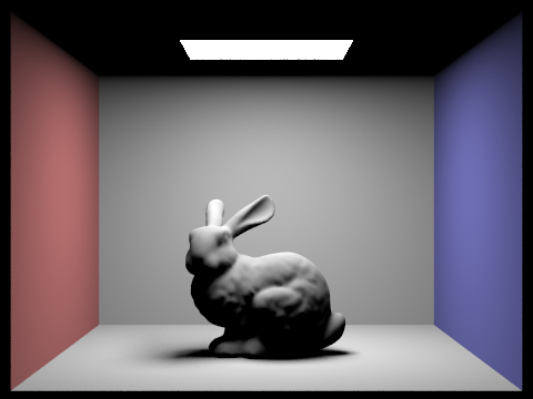
../dae/sky/CBbunny.dae, 64 samples per pixel
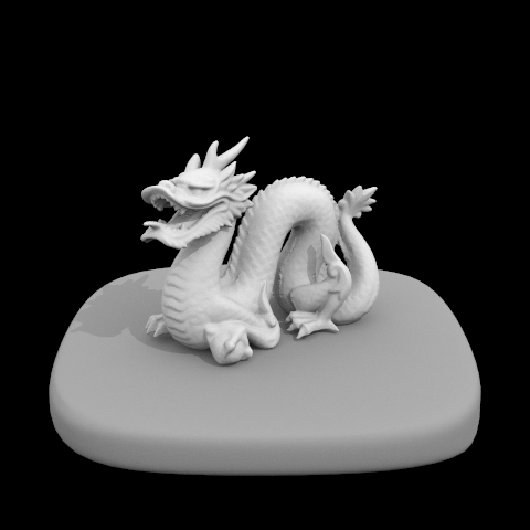
../dae/sky/dragon.dae
Using light importance sampling, we can also compare the noise levels in soft shadows when rendering with 1, 4, 16, and 64 light rays (the -l flag) and 1 sample per pixel (the -s flag) for ../dae/sky/CBbunny.dae. When there are more light rays, we can see that there is less noise in the rendered images. The shadows become more smooth and the edges are less rigid because with less light rays, each shadow point is clearer. With more light rays, there is a greater range, allowing for more variation in the shadows.
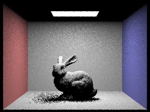
../dae/sky/CBbunny.dae, 1 light ray

../dae/sky/CBbunny.dae, 4 light rays

../dae/sky/CBbunny.dae, 16 light rays

../dae/sky/CBbunny.dae, 64 light rays
Uniform Hemisphere Sampling vs Light Sampling
As seen in the images below, lighting sampling results in smoother and sharper images whereas uniform hemisphere sampling results in grainier/noisier images. This is a result of uniform hemisphere sampling taking samples in different directions around a given point, thus causing some areas to be darker/grainer. Lighting sampling samples from the light source - samples that actually affect the final lighting. By doing this, we remove noise because not all samples of hemisphere sampling were not in the direction of the light source.
Uniform Hemisphere Sampling

../dae/sky/CBbunny.dae with uniform hemisphere sampling
Direct Lighting Sampling

../dae/sky/CBbunny.dae with direct lighting sampling
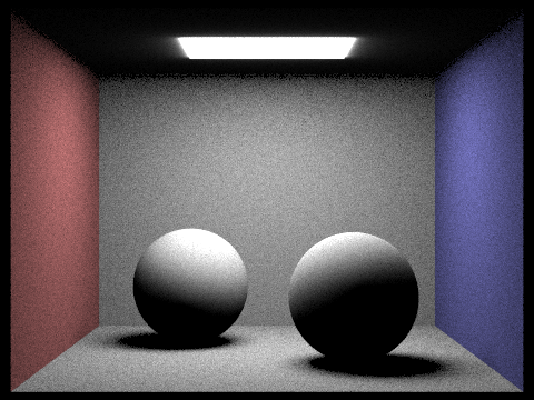
../dae/sky/CBlambertian_spheres.dae with uniform hemisphere sampling

../dae/sky/CBlambertian_spheres.dae with direct lighting sampling
Part 4: Global Illumination
Task 1: Sampling with Diffuse BSDF
Task 2: Global Illumination with up to N Bounces of Light
Task 3: Global Illumination with Russian Roulette
Walk through your implementation of the indirect lighting function.
The purpose of indirect lighting is to take into account the reflecting light at a certain point from other objects instead of exclusively light sources. In our implementation, we updated est_radiance_global_illumination to return L_out as the sum of the calls to zero_bounce_radiance and at_least_one_bounce_radiance. Based on the spec, we also changed the camera ray's depth to be max_ray_depth.
If the ray's depth is equal to 0, we just return Vector3D(0, 0, 0). Otherwise, if the ray's depth is greater than 1, we recursively call one_bounce_radiance when tracing backwards through the incoming light vectors. We generate a sample Ray from hit_p and ray_dir (o2w * w_in). We set the ray's min_t to EPS_F and the max_t to r.depth - 1 as outlined in the spec. This enables us to be able to decrement the depth for each bounce performed.
We check whether nodes in our BVH intersect the sample ray and if so, we calculate new_L (\( L_i\)) which is a recursive call to at_least_one_bounce_radiance and we also calculate \( \cos(\theta_j)\). Each intersection is scaled by the appropriate lambert term and pdf (and cdf for Russian Roulette). We accumulate L_out as \( \frac{{L_i \times f_r \times \cos(\theta_j)}}{{\text{pdf}}} \) and return it at the end.
Each intersection is scaled by the appropriate lambert term and pdf (and cdf for Russian Roulette). If an intersection isn't found, we just return the radiance at the current iteration and pop back up. We recurse until the maximum ray depth or if Russian Roulette is enabled, it would terminate with a 0.35 chance.
To account for non-accumulated bounces, if isAccumBounces = false, we only add the outgoing light for the last bounce and for other bounces, we return Vector3D(0, 0, 0). Within our code, if isAccumBounces is true, we add one_bounce_radiance to L_out, representing us hitting the last bounce or if the ray's depth is one. If there is an intersection and isAccumBounces = false, we don't accumulate to L_out but instead set L_out equal to \( \frac{{L_i \times f_r \times \cos(\theta_j)}}{{\text{pdf}}} \).
For Russian Roulette, when the ray's depth is greater than 1, we take a coin_flip and pass in a probability of 0.65 since our termination probability is 0.35. If the coin_flip is true, we recurse.
Show some images rendered with global (direct and indirect) illumination. Use 1024 samples per pixel.

../dae/sky/CBlambertian_spheres.dae with global illumination
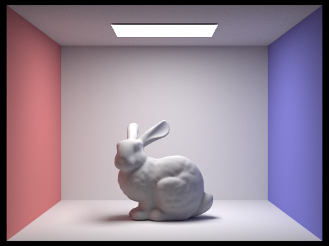
../dae/sky/CBbunny.dae with global illumination
Pick one scene and compare rendered views first with only direct illumination, then only indirect illumination. Use 1024 samples per pixel. (You will have to edit PathTracer::at_least_one_bounce_radiance(...) in your code to generate these views.)
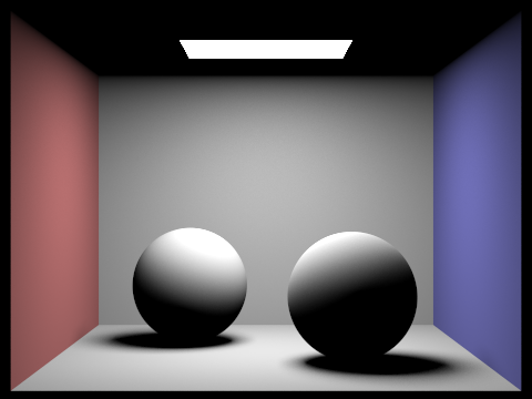
../dae/sky/CBlambertian_spheres.dae with only direct illumination
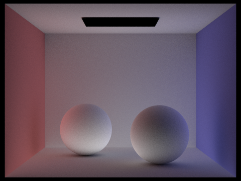
../dae/sky/CBbunny.dae with only indirect illumination
Direct illumination consists of zero-bounce and one-bounce illumination, whereas indirect illumination incorporates two or more bounces.
For CBbunny.dae, render the mth bounce views of light with max_ray_depth set to 0, 1, 2, 3, 4, and 5 (the -m flag). Also compare rendered views with accumulation on, with max_ray_depth set to 0, 1, 2, 3, and 5 (the -m flag). Use 1024 samples per pixel.
No Accumulation

../dae/sky/CBbunny.dae, zero bounces of light
With Accumulation
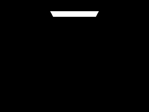
../dae/sky/CBbunny.dae, zero bounces of light
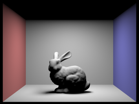
../dae/sky/CBlambertian_spheres.dae, one bounce of light

../dae/sky/CBlambertian_spheres.dae, one bounce of light
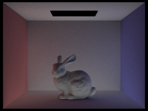
../dae/sky/CBlambertian_spheres.dae, two bounces of light

../dae/sky/CBlambertian_spheres.dae, two bounces of light
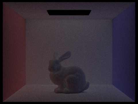
../dae/sky/CBlambertian_spheres.dae, three bounces of light

../dae/sky/CBlambertian_spheres.dae, three bounces of light
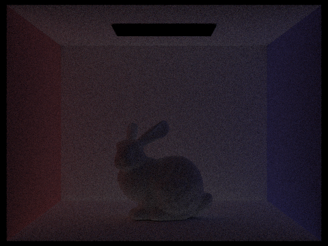
../dae/sky/CBlambertian_spheres.dae, four bounces of light

../dae/sky/CBlambertian_spheres.dae, four bounces of light
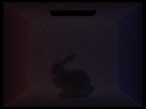
../dae/sky/CBlambertian_spheres.dae, five bounces of light

../dae/sky/CBlambertian_spheres.dae, five bounces of light
Based on the images above, we are able to see that adding bounces of light with global illumination causes images to look more "realistic" since shadows (complex and diffuse) and colors are displayed more evidently in the iamges. We can see that between the second and third bounce of light, the image gets substantially darker. This is because after the second bounce, the light has dissipated. There is still a bit of light around the bunny's legs because after the second bounce of light, light that hits the ground would hit the bunny's legs. Subsequent bounces only light the edges of the floor and slightly under the bunny. The decreased light can also be a result of absorption from the walls.
Pick one scene and compare rendered views with various sample-per-pixel rates, including at least 1, 2, 4, 8, 16, 64, and 1024. Use 4 light rays.
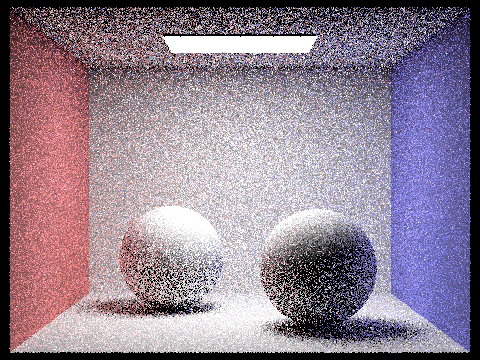
../dae/sky/CBlambertian_spheres.dae, 1 sample per pixel, 4 light rays
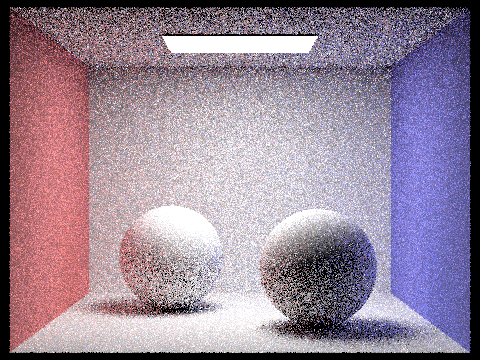
../dae/sky/CBlambertian_spheres.dae, 2 samples per pixel, 4 light rays
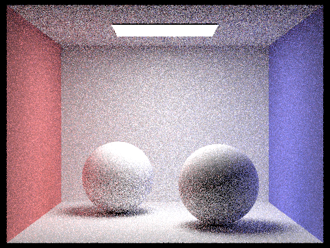
../dae/sky/CBlambertian_spheres.dae, 4 samples per pixel, 4 light rays
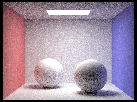
../dae/sky/CBlambertian_spheres.dae, 8 samples per pixel, 4 light rays

../dae/sky/CBlambertian_spheres.dae, 16 samples per pixel, 4 light rays
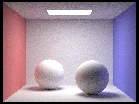
../dae/sky/CBlambertian_spheres.dae, 64 samples per pixel, 4 light rays
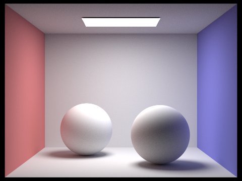
../dae/sky/CBlambertian_spheres.dae, 1024 samples per pixel, 4 light rays
Based on the images above, we can see that with a greater pixel sampling rate, the bunny image gets less grainier/noisy and becomes clearer and smoother. This is a result of higher sampling rates which eliminates noise.
For CBbunny.dae, compare rendered views with accumulation on, while using Russian Roulette, with max_ray_depth set to 0, 1, 2, 3, and 100 (the -m flag). Use 1024 samples per pixel.
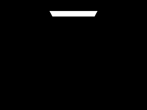
../dae/sky/CBbunny.dae, max_ray_depth = 0 with Russian Roulette
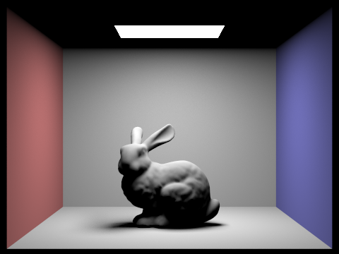
../dae/sky/CBbunny.dae, max_ray_depth = 1 with Russian Roulette
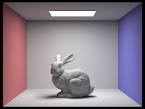
../dae/sky/CBbunny.dae, max_ray_depth = 2 with Russian Roulette

../dae/sky/CBbunny.dae, max_ray_depth = 3 with Russian Roulette

../dae/sky/CBbunny.dae, max_ray_depth = 4 with Russian Roulette

../dae/sky/CBbunny.dae, max_ray_depth = 100 with Russian Roulette
The purpose of Russian Roulette is to allow for unbiased termination in the recursive model for outgoing light at different bounces. With Russian Roulette implemented, the images are brighter with increased color bleeding in the shadows and maximum ray depth. However, we noticed that there isn't a significant difference between max_ray_depth = 4 and max_ray_depth = 100. This is most likely a result of Russian Roulette random termination since there is a 0.3 probability of termination at each level of recursion, indicating that the image probably didn't reach 100 levels of bounces.
Part 5: Adaptive Sampling
Explain adaptive sampling. Walk through your implementation of the adaptive sampling.
The purpose of adaptive sampling is to decrease the number of samples per pixel (per pixel basis) which makes the Monte Carlo path tracing more efficient. This is done by checking if a pixel has a variance within an acceptable range. If so, sampling will be terminated there. Ultimately, it concentrates samples in areas that are more difficult to render.
This builds off of what we did in Part 1 Task 2. As noted in the spec, we want \( I \leq \text{maxTolerance} \times \mu \) where \( \mu = 1.96 \times \left(\frac{{\text{SD}}}{{\sqrt{n}}}\right) \). \(\mu\) represents the current mean illuminance, and \(SD\) is the standard deviation of the illuminances for the samples that have already been taken. We don't need to keep track of every sample's illuminance - we just keep track of \( s_1 = \sum_{k=1}^{n} x_k \) and \( s_2 = \sum_{k=1}^{n} x_k^2 \). This allows us to recover \(\mu = \frac{{s_1}}{n} \) and \(\sigma^2 = \frac{1}{{n-1}} \times \left(s_2 - \frac{{s_1^2}}{n}\right) \).
Mainly where iterating through num_samples times, we check whether adaptive_num_samples (index i) is a multiple of samplesPerBatch. If so, we perform a convergence check which is elaborated above and in the spec. When \( I \leq \text{maxTolerance} \times \mu \), we can assume that the pixel has converged, allowing us to stop tracing more rays. However, if the pixel hasn't converged, we obtain a sample and normalize the sample within the pixel. We do this by generating a Ray and calling est_radiance_global_illumination to add to vec_sum (overall pixel's radiance). We add to s1 and the squared value to s2. Once the iteration is complete, we normalize the pixel's average radiance (vec_sum), call update_pixel, and update sampleCountBuffer.
Pick two scenes and render them with at least 2048 samples per pixel. Show a good sampling rate image with clearly visible differences in sampling rate over various regions and pixels. Include both your sample rate image, which shows your how your adaptive sampling changes depending on which part of the image you are rendering, and your noise-free rendered result. Use 1 sample per light and at least 5 for max ray depth.

../dae/sky/CBbunny.dae, rendered image
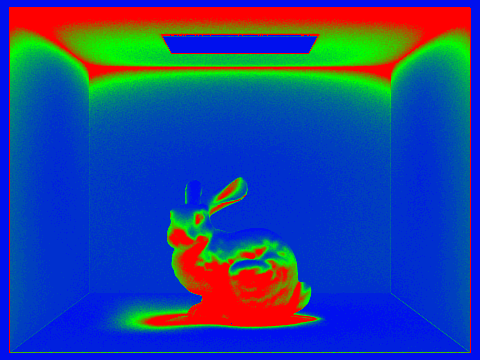
../dae/sky/CBbunny.dae, sample rate image
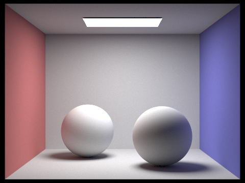
../dae/sky/CBlambertian_spheres.dae, rendered image
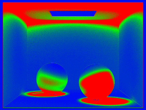
../dae/sky/CBlambertian_spheres.dae, sample rate image
We notice that the red color represents high sampling rates while the blue color represents low sampling rates.