CS184/284A Spring 2026 Homework 2

Link to webpage: Github webpage
Link to GitHub repository: github.com/cal-cs184-student/hw2-meshedit-corgi

Overview

This homework, we implemented Bezier curves and surfaces, and also triangle meshes and modifications. First, we worked on using de Casteljau’s algorithm to create Bezier curves, and we were able to easily apply that to make Bezier surfaces. Then, we got familiar with the half edge data structure, and used the data structure to implement area-weighted area normals (which was used for smooth shading), edge flips and split edges in triangle meshes, and finally tie that all together to implement loop subdivision for mesh sampling (which generates smoother surfaces).

The coolest thing we worked on was probably the half edge mesh implementation. When looking through the halfEdgeMesh.h file, it seemed pretty straightforward and simplistic, but our full implementation practically hinged on understanding the data structure, and it was cool how we were able to perform all these operations with just half edges (and other elements, but those were defined mainly by half edges too).

Also, we learned about how upsampling helps render smoother surfaces. It helped us understand how to improve resolution, but also how we can manipulate the mesh for clarity despite not having extra information. It seemed like a pretty useful technique that hopefully we will learn more about in the future.

Overall, this project was helpful in implementing what we’ve learned in lecture, and is a great rendering tool.

Section I: Bezier Curves and Surfaces

Part 1: Bezier curves with 1D de Casteljau subdivision

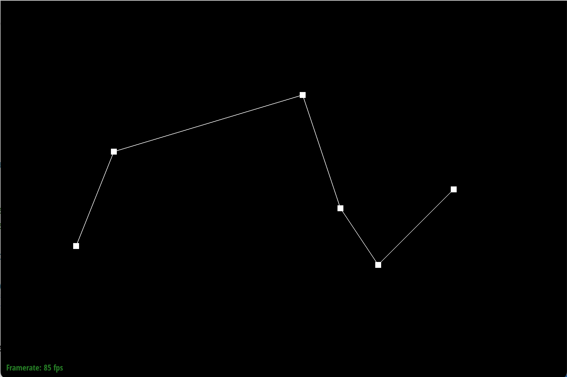
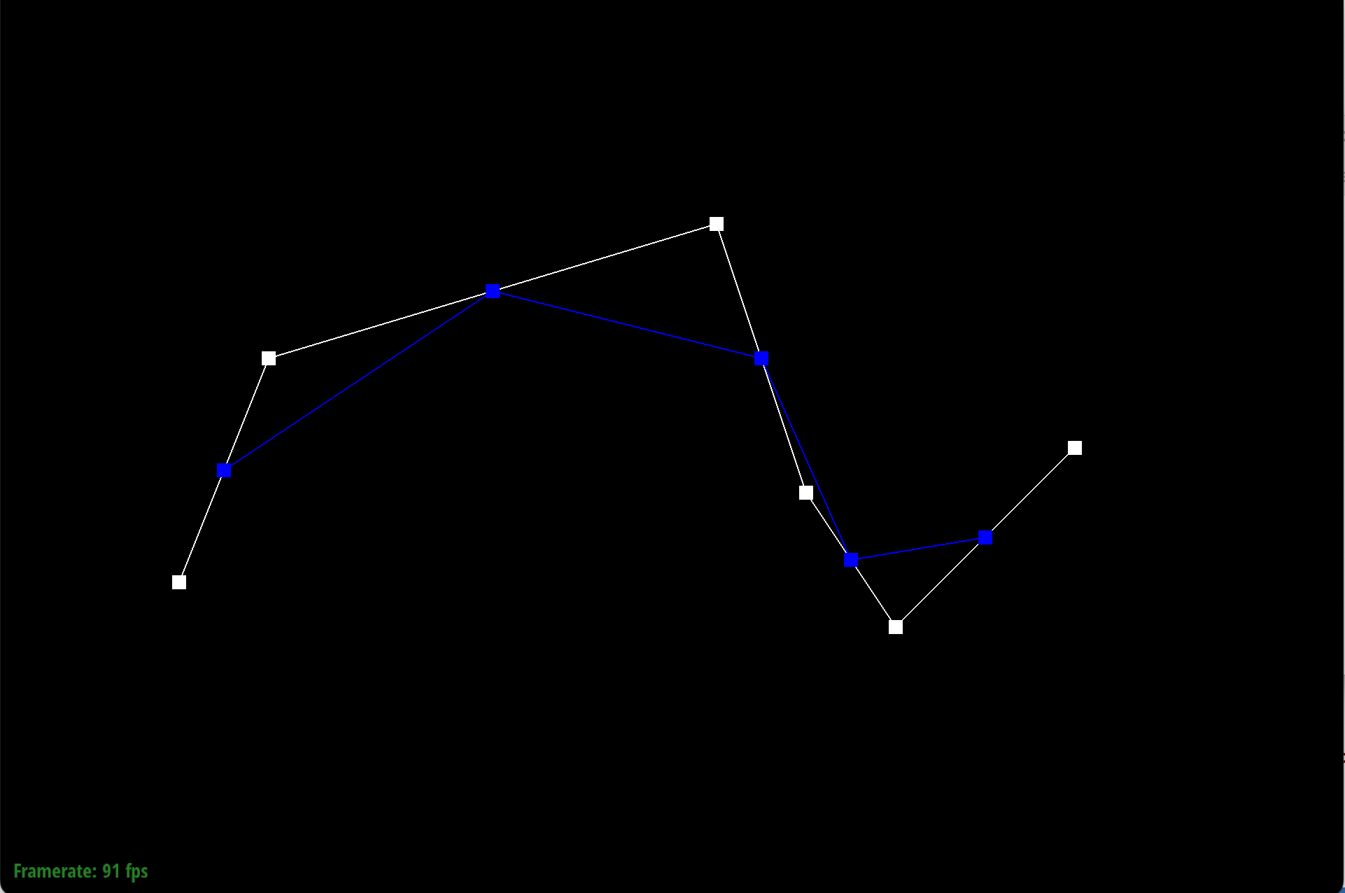
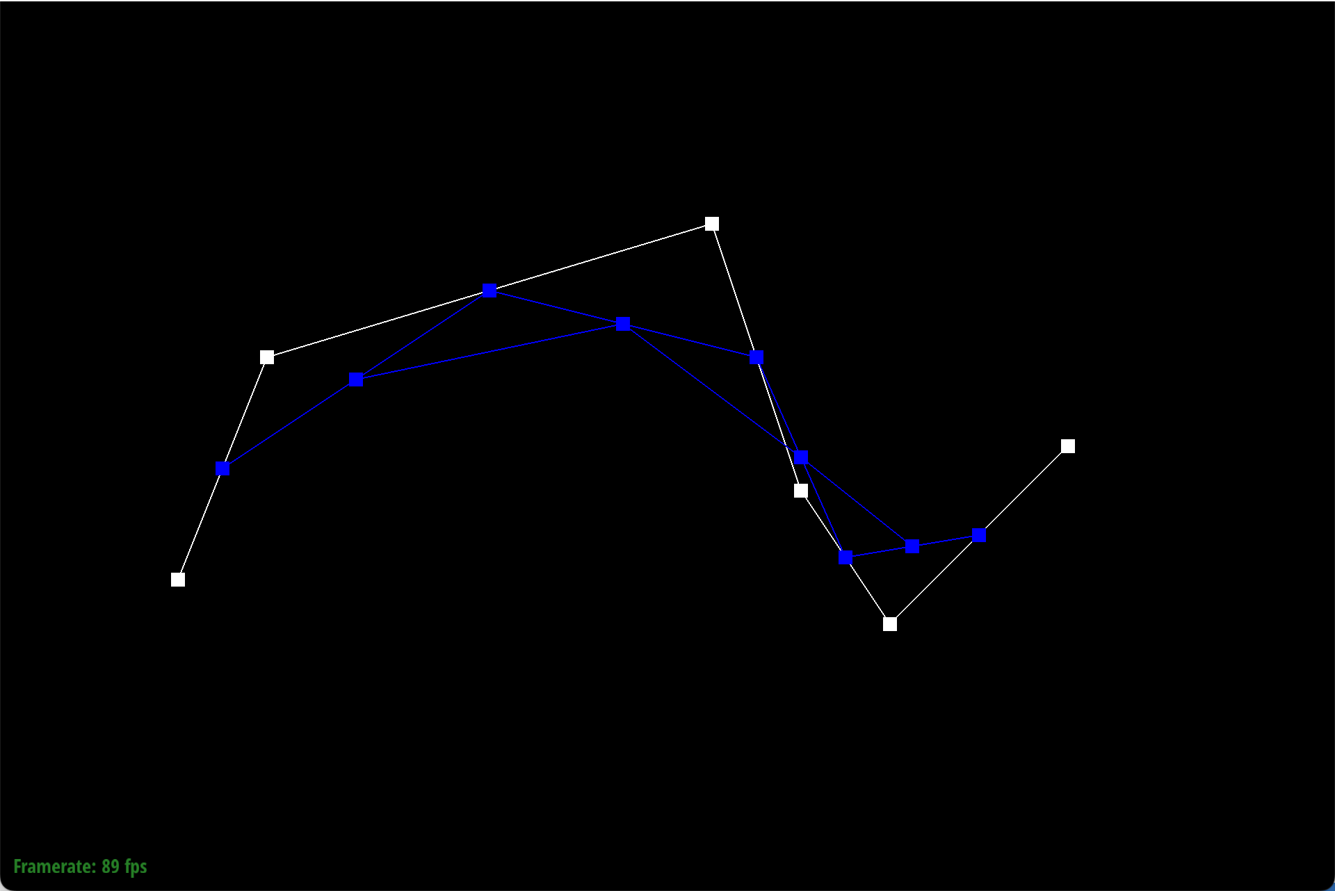
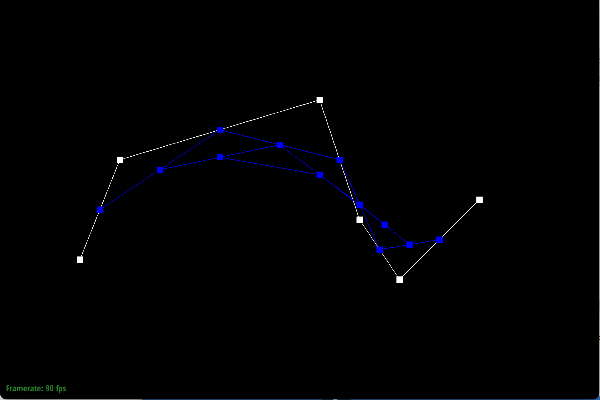
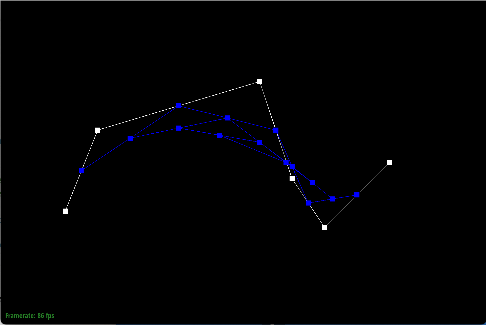
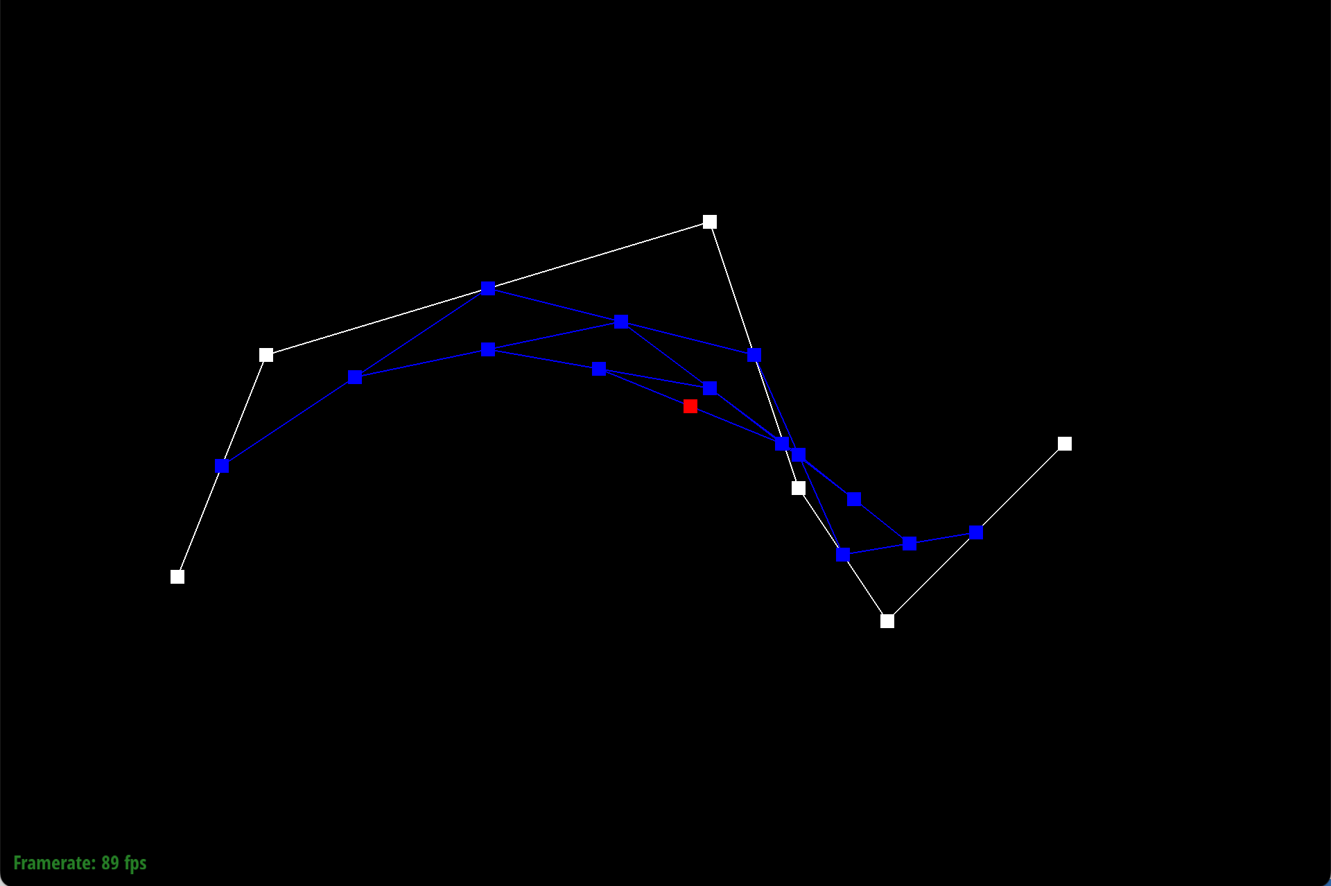
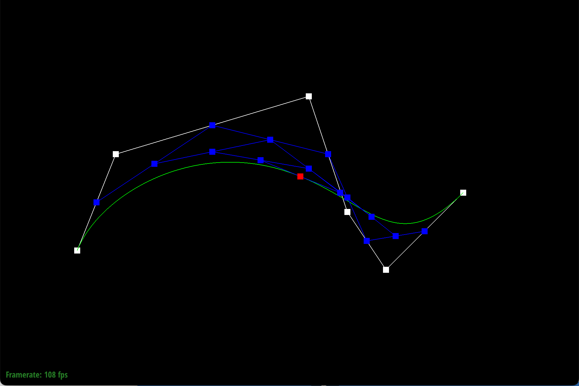
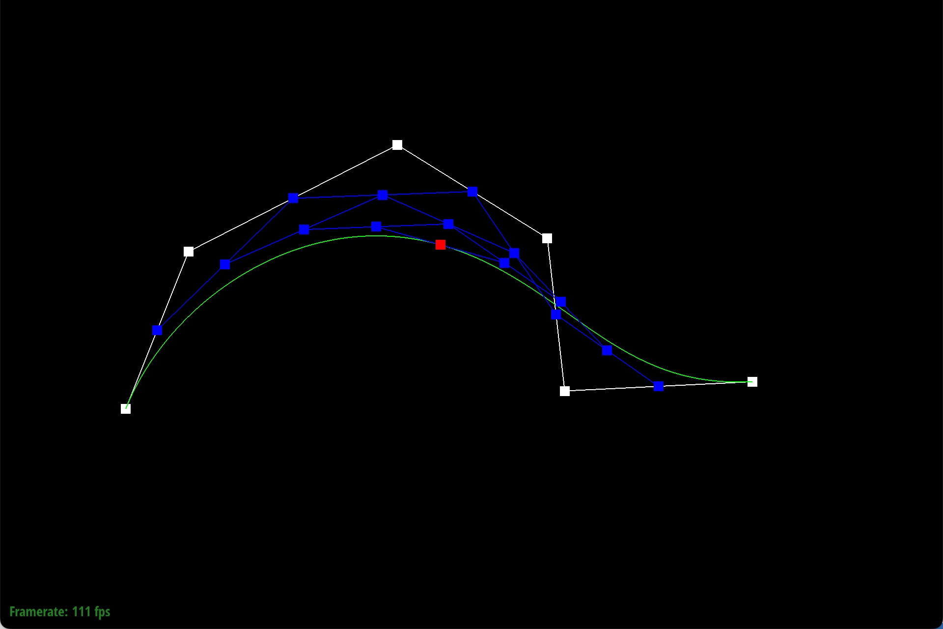
The de Casteljau's algorithm is essentially repeated linear interpolation on subsets of points. Our method performs one step, aka one linear interpolation for each pair of adjacent points. Given two points, we will insert a point on the line between them using linear interpolation. So the formuala we used was \((1-t)*p_i + t*p_j\), where t is the parameter given by the BezierCurve class, and \(p_i\) and \(p_j\) are two adjacent points. In order to fully evaluate the curve, two things must be done.

1. We need to perform these linear interpolations on all the adjacent pairs of points in the original control points, and returned the outputs.
2. Repeat step 1 on the new outputted points. Eventually, you will receive a single point, the product of all the linear interpolations.

Our method performs step 1 once, but you can use the GUI to perform it repeatedly until you get the final point and curve.

Here is each step/level of the evaluation using de Casteljau.

Part 2: Bezier surfaces with separable 1D de Casteljau

de Casteljau algorithm takes in a set of points, or a 1D vector. To extend this to Bezier surfaces, on a 2D m by n vector, we perform de Casteljau on each row or entry of points, using a certain parameter u. Then we will receive n points as output from this, and we will perform de Casteljau one final time with a parameter v on these output points. This will give us our Bezier surface.

We implemented this in three parts:

1. First we created a method evaluateStep to evaluate one step of the de Casteljau algorithm using the given points and the scalar parameter t. This is simply the linear interpolations.
2. Then, we created a method evaluate1D that fully evaluates de Casteljau for a vector of points at scalar parameter t. This method just calls our evaluateStep method m - 1 times (where m is the number of points in our vector).
3. Finally, we implemented the evaluate method, which evaluates the Bezier patch at parameter (u, v). To do this, we call evaluate1D for each vector in the control points using parameter u. Then, we call evaluate1D on those outputs using parameter v.

Section II: Triangle Meshes and Half-Edge Data Structure

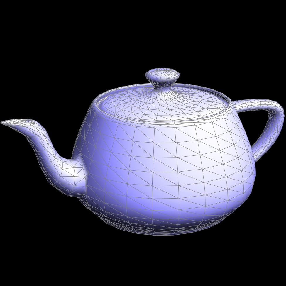
Part 3: Area-weighted vertex normals

To implement the area-weighted vertex normals, we had to iterate through the faces who share the vertex, and for each face, weight its normal by the face area, and then finally normalize the sum of all the area-weighted normals. To do this, we kept track of the area-weighted normal sum. Then, we iterated through the half-edges of the vertex. At each iteration, we got the corresponding face (since each half-edge has its face), and then got the normal using the already-implemented normal function. Then we calculated the area of the face using the formula \(1/2 * ||normal||\). Finally we calculated the weighted normal by multiplying the normal and area, and then added that vector to the sum vector. At the very end, we returned the normalized sum.

Part 4: Edge flip

To implement the edge flip operation, it helped a lot to draw out what two neighboring triangles would look like before and after an edge flip. This way, we could keep track of what elements we actually would need to change.

In our code, first, we checked if either of our faces were on a boundary loop. If not, then we proceeded to keep track of all the pointers and elements that we may need in our edge flip. So we kept pointers to the two main half edges, h1 and h2, as well as their next elements, as well as their next next elements. Essentially the half edges that currently kept track of the two triangles. We also kept track of the vertices.

Then, we started reassigning. Mainly, we reassigned the vertices of h1 and h2. We adjusted the next pointers and the twin pointers. This got pretty buggy, because at first we were just reassigning the next edges of our two main half edges h1 and h2, but once we started keeping track of our original next elements and original next next elements, we reassigned those pointers too, and were able to resolve the bugs. We also updated the other elements, like the faces, edges, and vertices, to point to our updated half edges. Finally, we returned our original edge.

Our debugging was mainly a combination of drawing out our half edges and also using the check_for debugging functions. These told us the address of elements and who pointed to them, and we used these to work on understanding the relationships and what we needed to fix.

Part 5: Edge split

To implement the edge split operation, we first created pointers to practically all the elements in the original mesh: the half edges, faces, edges, and vertices. Then, we created all the new elements using the newHalfedge() and other new methods. Next, we reassigned all the pointers for these new elements as well as for any existing elements. Finally, we deleted any elements that we no longer needed (like the old faces and the input edge and its half edges).

This time, we did not actually experience any bugs, because we first drew out everything entirely, with labels for all the elements. Then we drew what the expectation should be after we split the edges, again labeling all the elements. Following these two reference images of ours, we simply created elements and reassigned where necessary, and were able to successfully implement splitting edges.

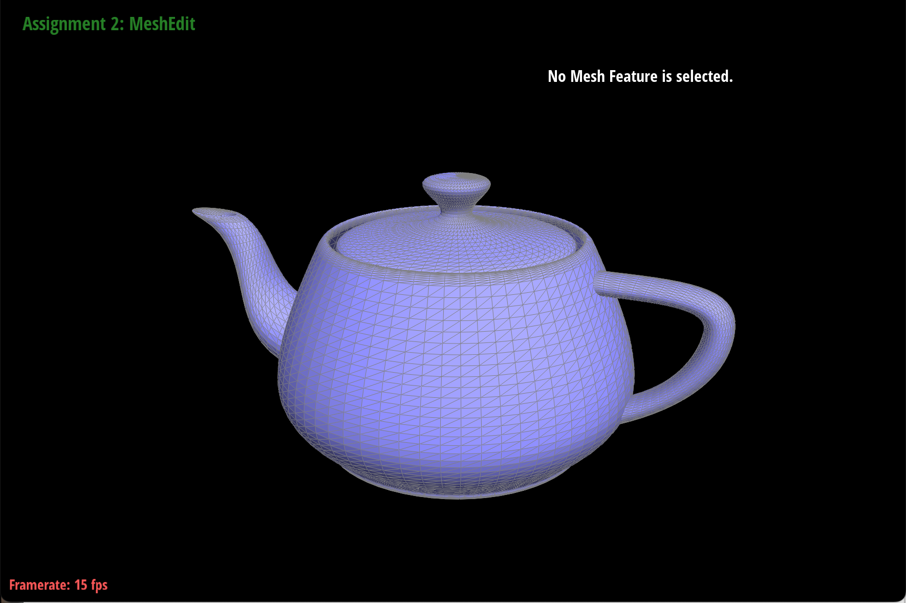
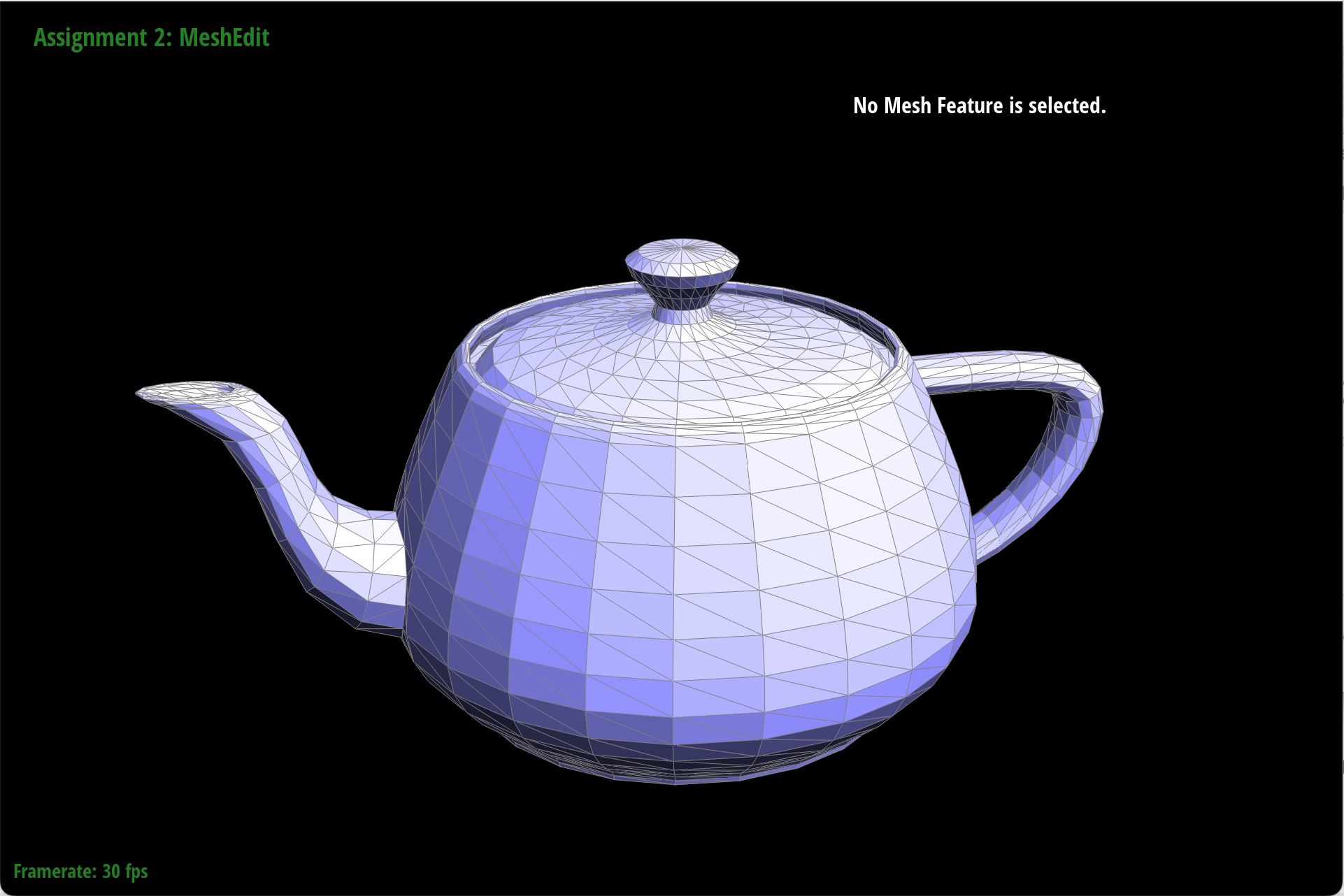
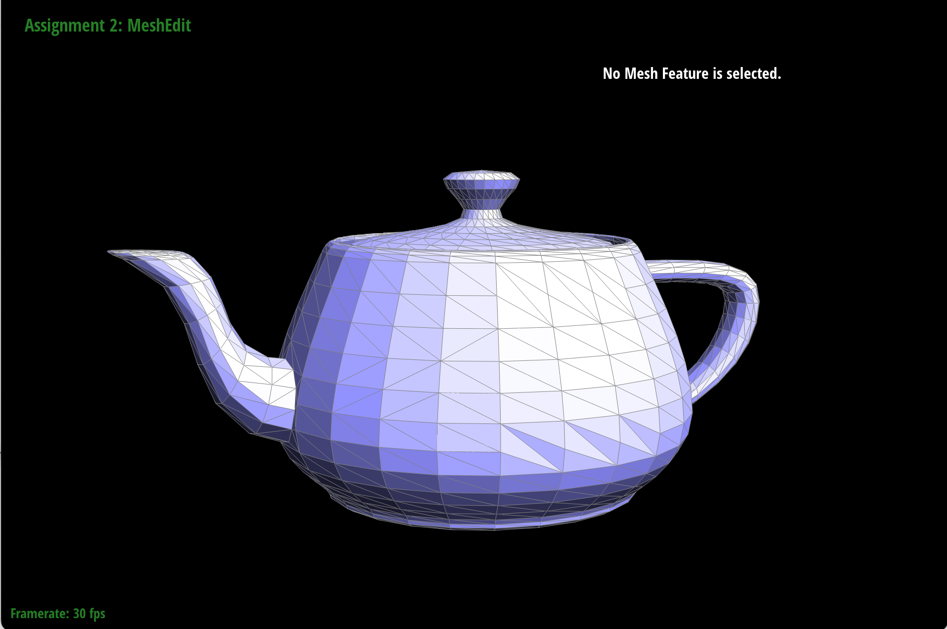
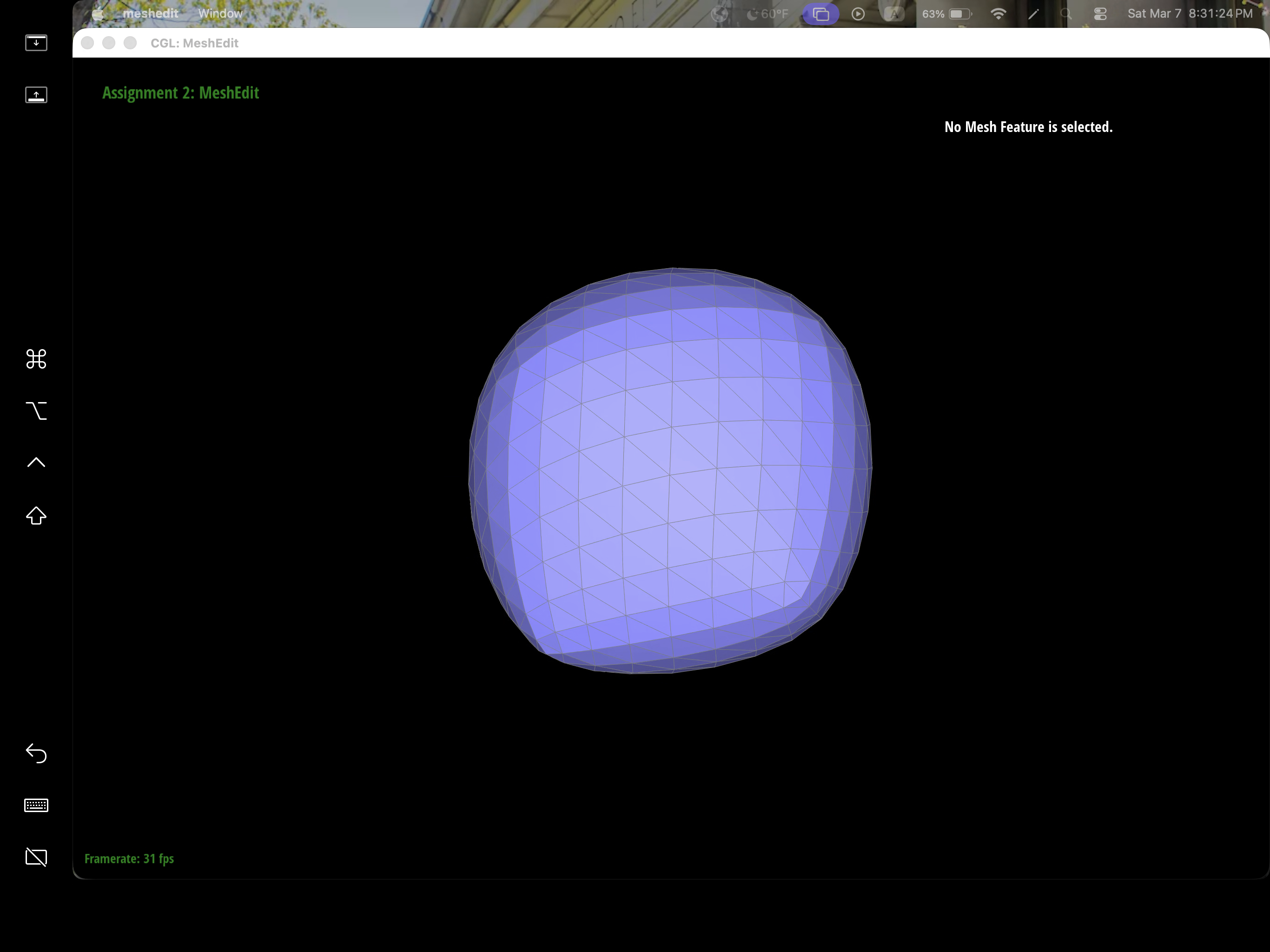
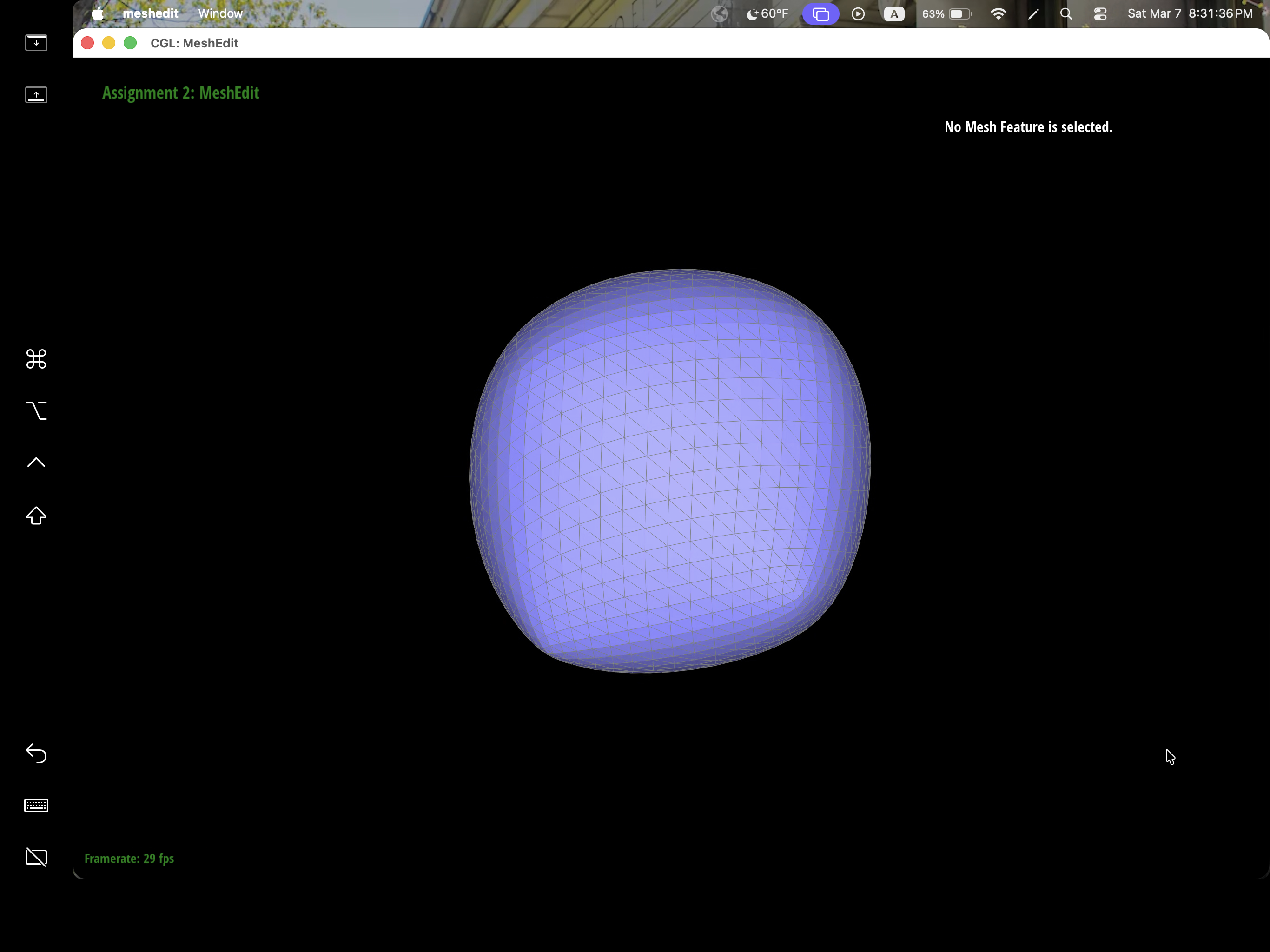
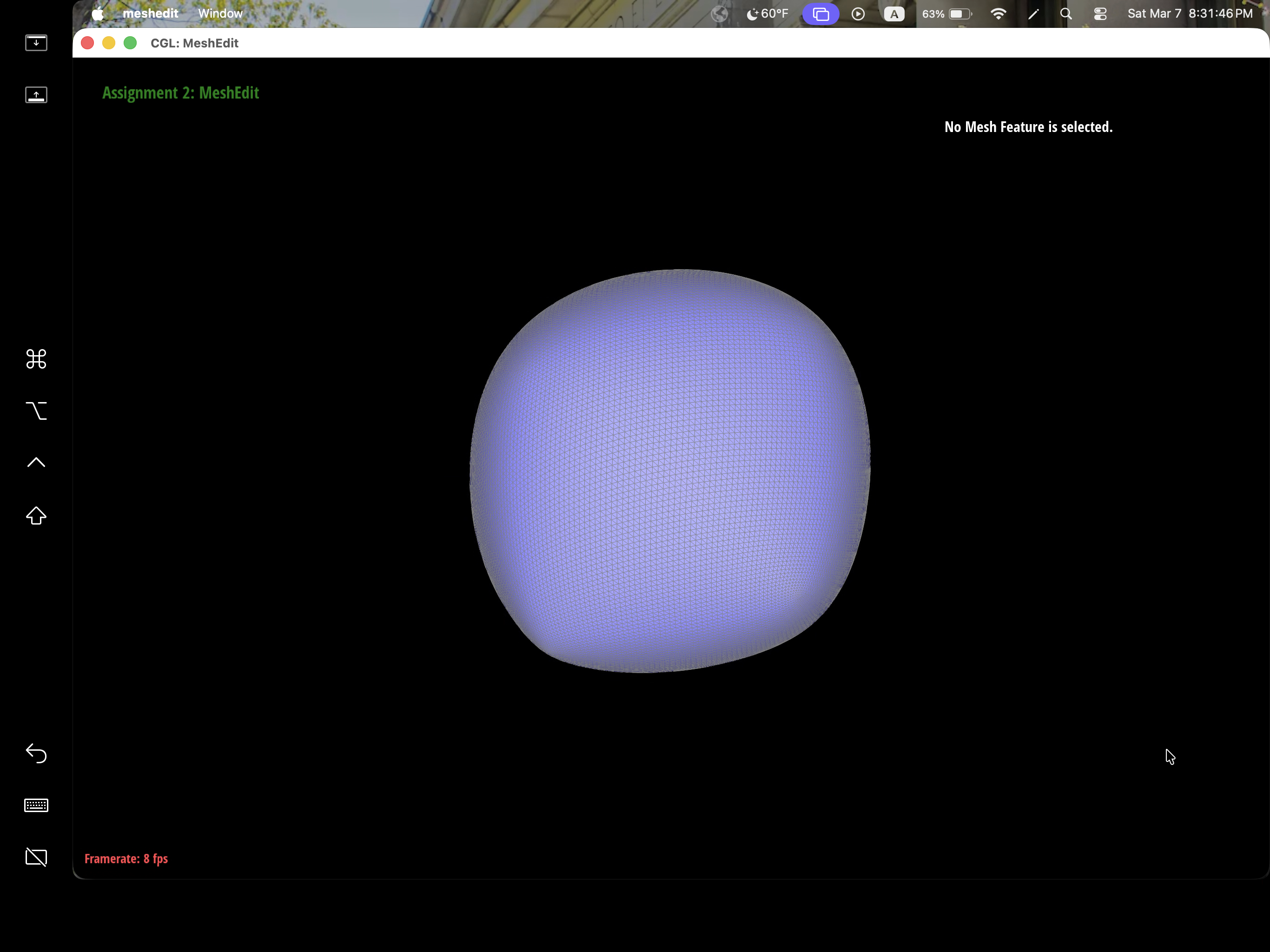
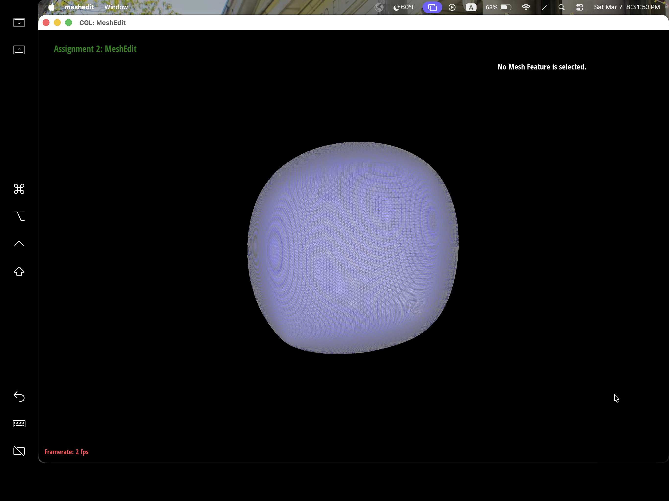
Part 6: Loop subdivision for mesh upsampling

To implement loop division, we proceeded in 5 steps.

1. We computed new positions for all the vertices in the input mesh via the loop subdivision rule, aka the old vertices. So we iterated through all the old vertices, and we used this rule: \((1-n*u) * og_pos + u * og_pos_sum\), where n is vertex degree, \(u = 3/16\) if \(n=3\), otherwise \(u=3/(8*n)\), og_pos is the original position of the old vertex, and og_pos_sum is the sum of all original positions of the neighboring vertices. To compute og_pos_sum, we iterated through neighboring vertices. The resulting computation we stored them in v->newPosition, and we marked each vertex as not new.
2. We computed the updated vertex positions associated with edges. We iterated through all the edges in the mesh. Using the edge, we computed what the new vertex position would be via this formula: \((3/8) *(A+B)+(1/8)*(C+D)\), where A, B, C, and D are the existing vertices associated with the edge. Then, we marked the edge as not new.
3. We split every edge in the mesh, in order. We iterated over the original mesh (to do this, we made a copy of the original mesh and iterated over that). Then, for each original edge, if the edge was not new, we split the edge, and assigned the position of the new vertex to be the one we had stored in step 2.
4. We flipped any new edge that connected an old and new vertex. We iterated through the edges, and if the edge is new, we checked if one associated vertex was old and one associated vertex was new, and if so, we flipped the edge.
5. Finally, for each vertex in our mesh, we assigned the vertex position to be the new position we had computed in steps 1 and 2.

Some debugging tricks we used was playing around with the vertex positions when implementing the new positions of edges to see how it affects the overall shape and thus determine if our approach was on the right line of logic or not.

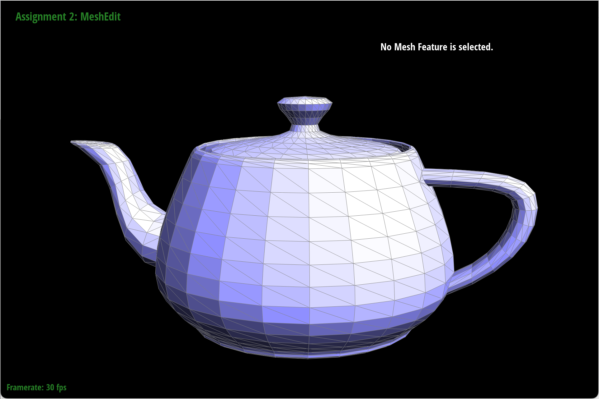
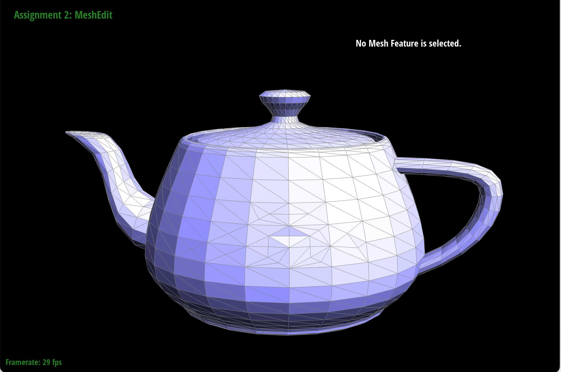
After loop subdivision, we notice that meshes become more smooth and rounded. The sharp corners and edges reduced to round edge and corners instead. This might be due to subdivision constantly averages the vertex position with their neighbors which throughout then smooths out the sharpness. This effect can be reduced by pre-splitting some edges to preserve sharp edges or corners.

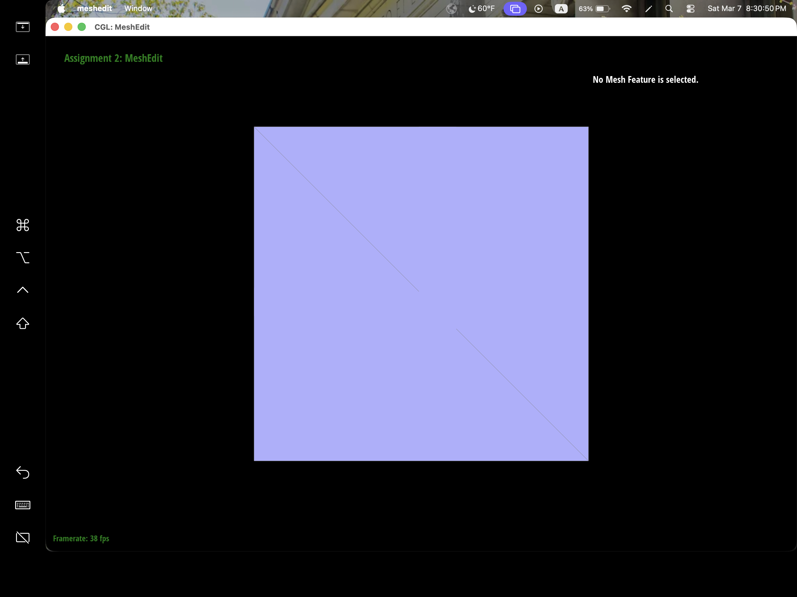
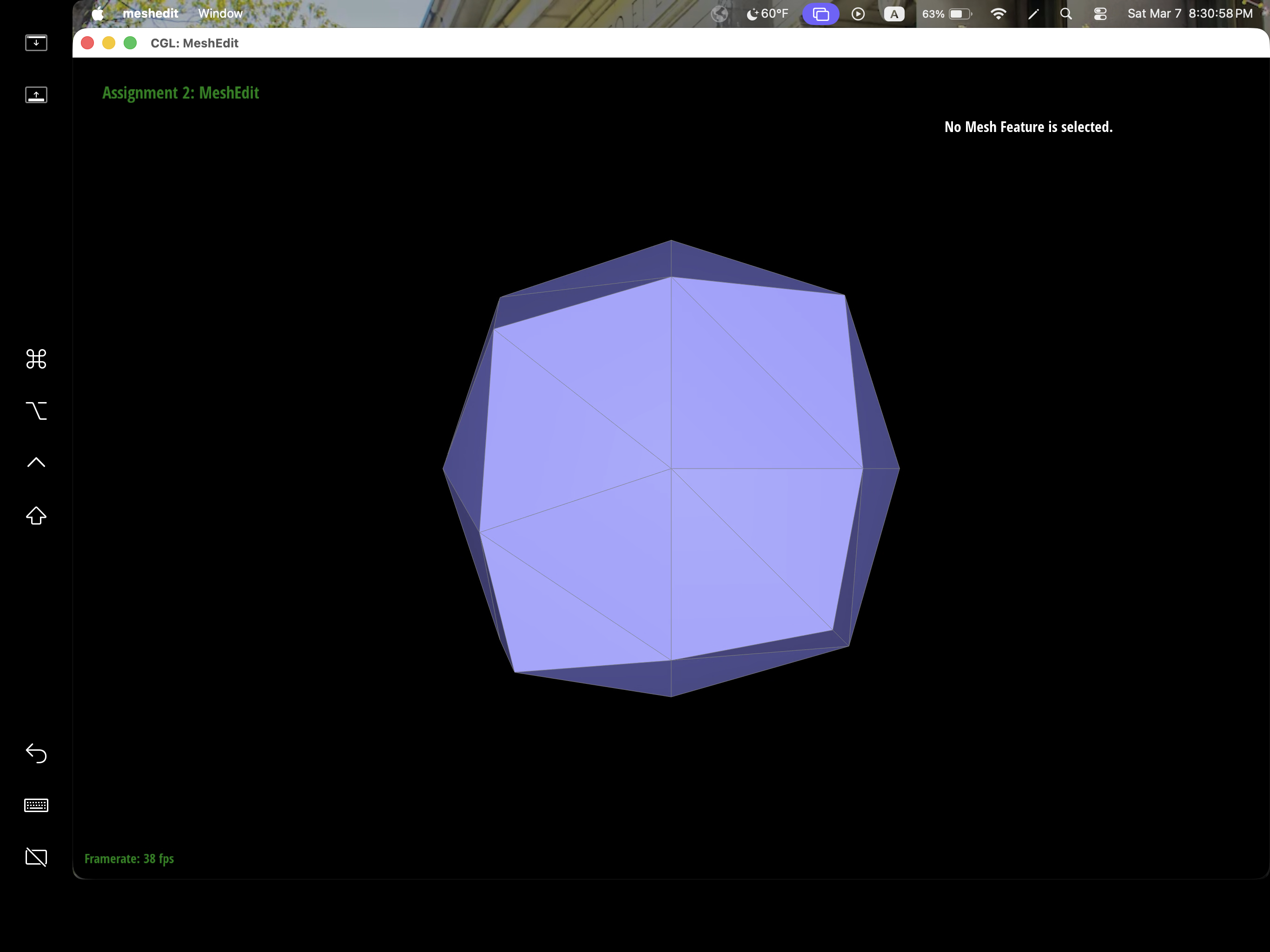
We can pre-process the cube with edge flips and splits so that the cube subdivides symmetrically. As the iterations of loop subdivision on the cube increases, so does the asymmetry since loop subdivision happens on the mesh's triangulation, the cube's face is then also triangulated with diagonals that might not exactly be symmetrical. Thus, when these asymmetries pile up over iterations, it becomes evident enough to look asymmetric. The pre-processing helps alleviate the effects because by flipping diagonals or performing edge splits, this allows the faces to have triangulations that match and thus have symmetry.