Stable Fluids Smoke

Jessie Liu, Luca Herden, Nada Hameed, Sarthak Agrawal

Link to webpage: cal-cs184-student.github.io/hw-webpages-nadahameed/final
Link to GitHub repository: github.com/jessieewoo/184-final-project
Video: Demo (Google Drive)
Presentation: Google Slides

Abstract

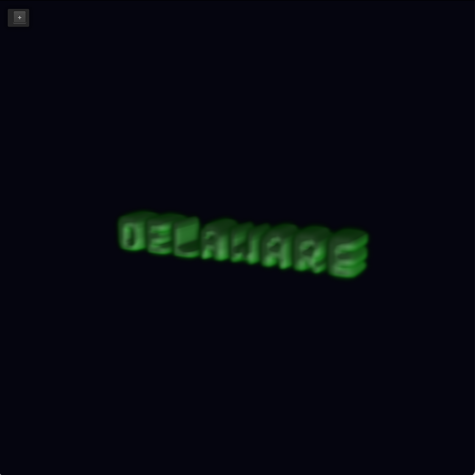
Our project is a 2D and 3D smoke simulator using stable fluids through Navier-Stokes. The smoke can emit from a certain shape, via hardcoded cells, typed text, or an imported image. Via the GUI, the user can control certain traits of the smoke: the emit rate (how much new smoke you inject each timestep at every emitter cell), the buoyancy (how strongly smoke rises), the decay rate (how fast smoke fades everywhere after each step), the color, and the strength of the cursor pushing on it. There are also a few toggles. Toggling '3' switches from 2D to 3D, and toggling 's' toggles fluid 3D and analytic 3D. The reason for the separate 3D versions is because fluid 3D is a bit more computationally intensive. We include an analytic implementation is included for sake of comparison, to show tradeoff between physical accuracy and cost/computation.

Technical approach

Implementation

Our implementation stemmed from HW4, cloth simulator. This was helpful because that already had a GUI in place we could use, as well as updating frames and rendering infrastructure. We just built on top of that with fluid simulation logic. We replaced the PointMass class with a FluidGrid class, and we replaced clothSimulator.cpp/h with smokeSimulator.cpp/h. There, we implemented our full rendering functionality, where FluidGrid was our solver.

2D

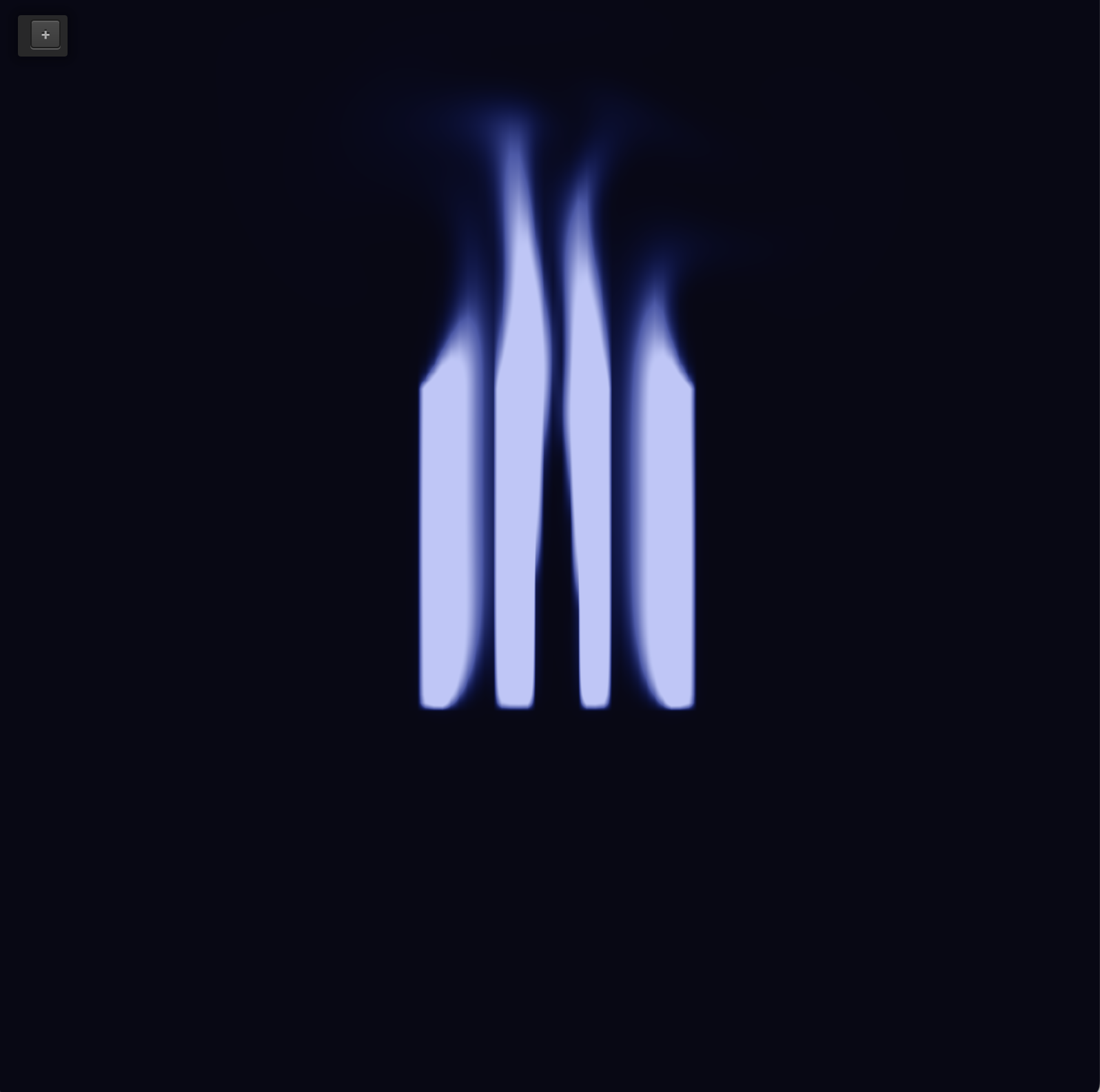
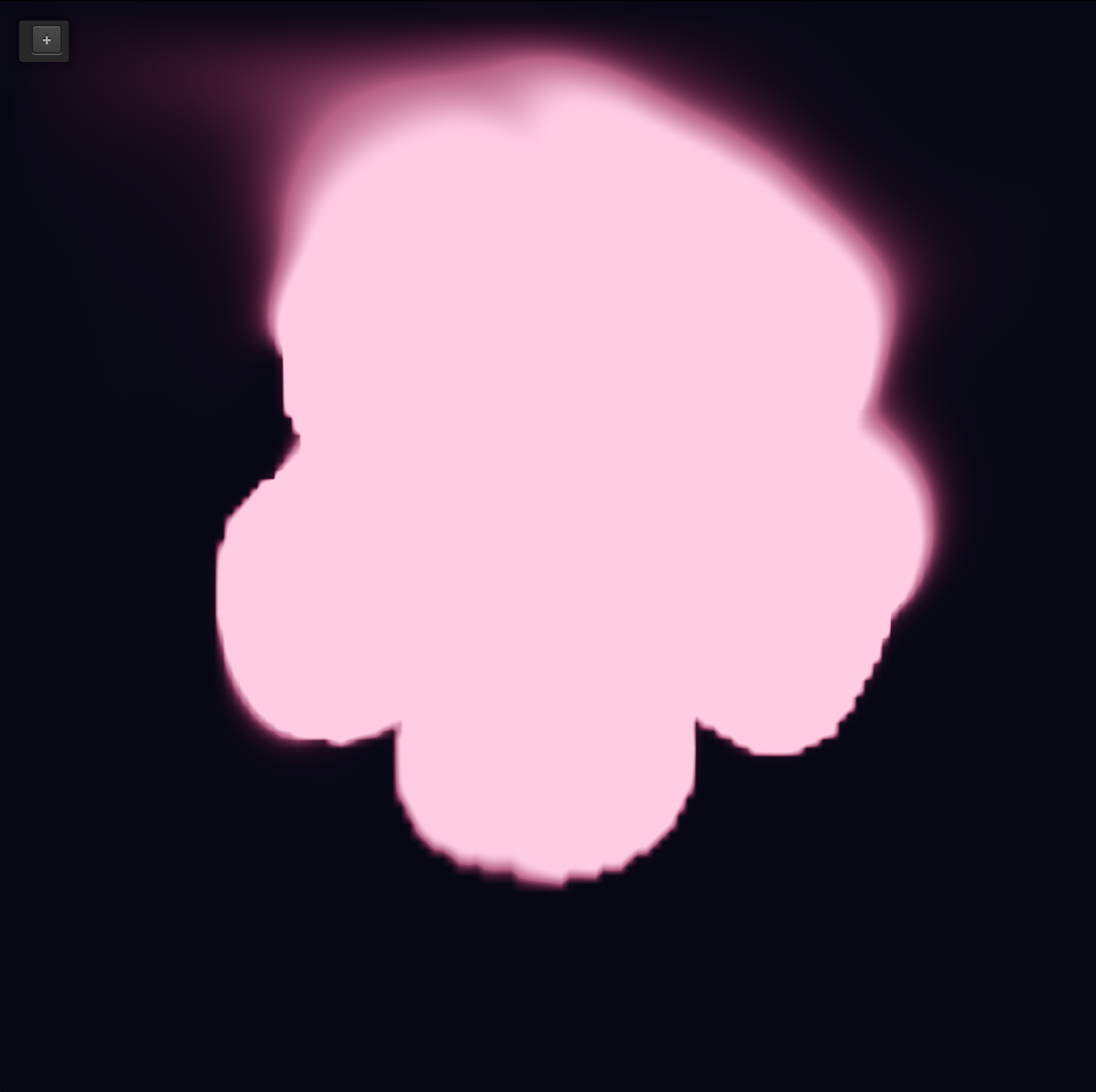
To implement 2D fluid simulation for our smoke, we created a grid of cells. Each cell keeps track of velocity (how fast the air is moving and in what direction), and how much smoke there is. Every frame, we add new smoke and wind, and then adjust and blend it with neighboring cells so that it looks like a real fluid and doesn't falsely compress or expand in each cell, and finally render the smoke density.

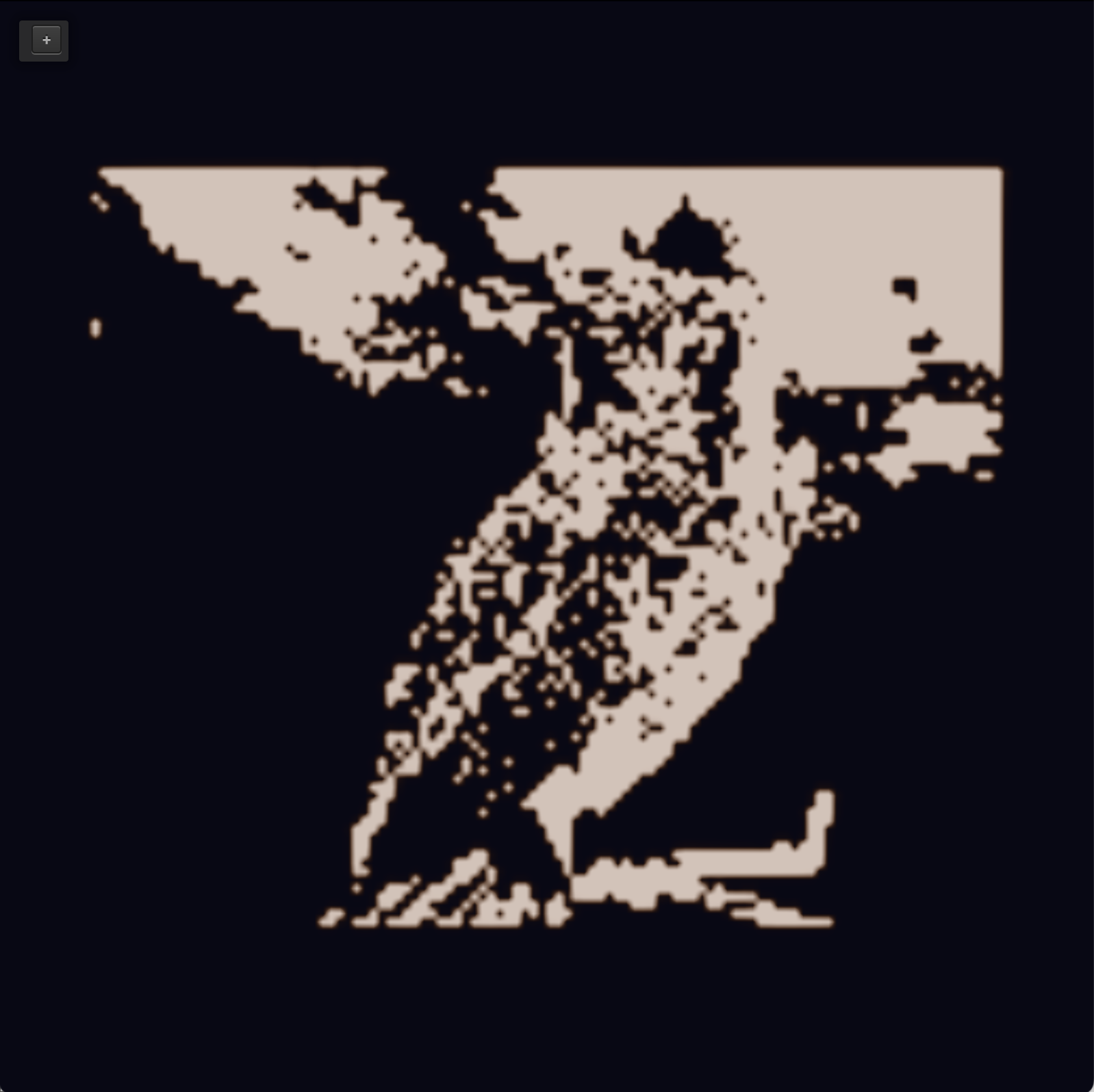
We used the fluid simulation implementation from Stam's paper Stable Fluids where we maintain a velocity field and a passive scalar (smoke field) on a cell-based grid. Each timestep, we update velocity via the Navier-Stokes equations and then update the movement of the density by that velocity. We have a class called LetterMask that determines which cells have smoke in them, ie which cells are on. We do this so that we can incorporate shapes into our simulation. This way, the smoke starts out in a certain input shape. We incorporate extra sources/forces based on user inputs in the GUI, like buoyancy. We also incorporate velocity from the mouse wind (which simulates pushing the smoke around).

3D analytic

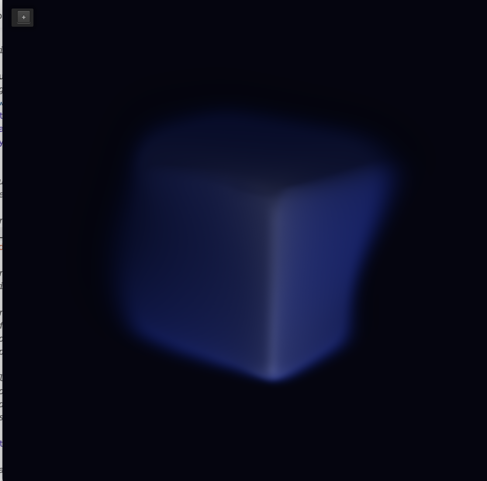
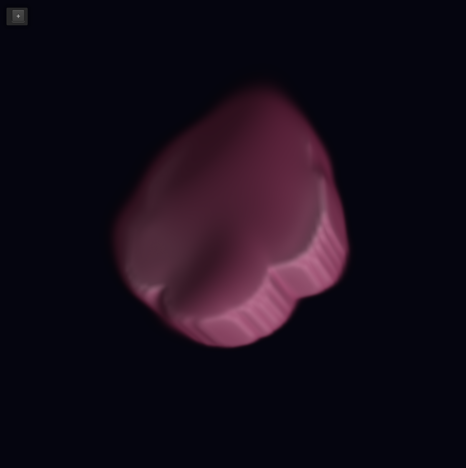
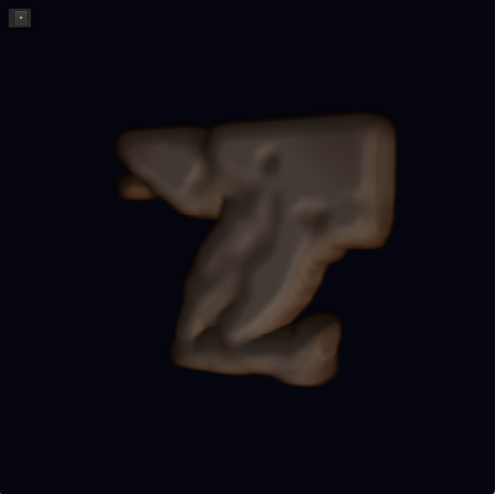
To implement 3D, we first implemented it analytically. In 2D, we solved for the wind every frame, following Stam's method. In 3D analytic, we do not run that heavy velocity solver. Instead, the wind at any point is solved using sine and cosine of position and time, plus an upward factor/force that scales with the buoyancy slider. So the smoke is designed to look swirly and modified over time, not produced by solving Navier-Stokes on the grid. When we say analytic, we mean that the wind is an explicit field that we can evaluate, not a simulated velocity field that is advanced every time step. The smoke still moves in a believable way, but it is far less computationally heavy. Every step, we carry velocity along that wind, then add new smoke near emitters, lightly blur with neighbors (so it looks smooth), and then fade with decay rate. To render 3D in our simululation, we draw a 3D density texture: the fragment shader does ray marching (taking many samples through the volume) so the screen shows thickness and depth, not a single flat image. For each pixel, the shader iterates through the volume and builds up color and opacity, which makes the smoke look thick and layered.

3D via Stam's

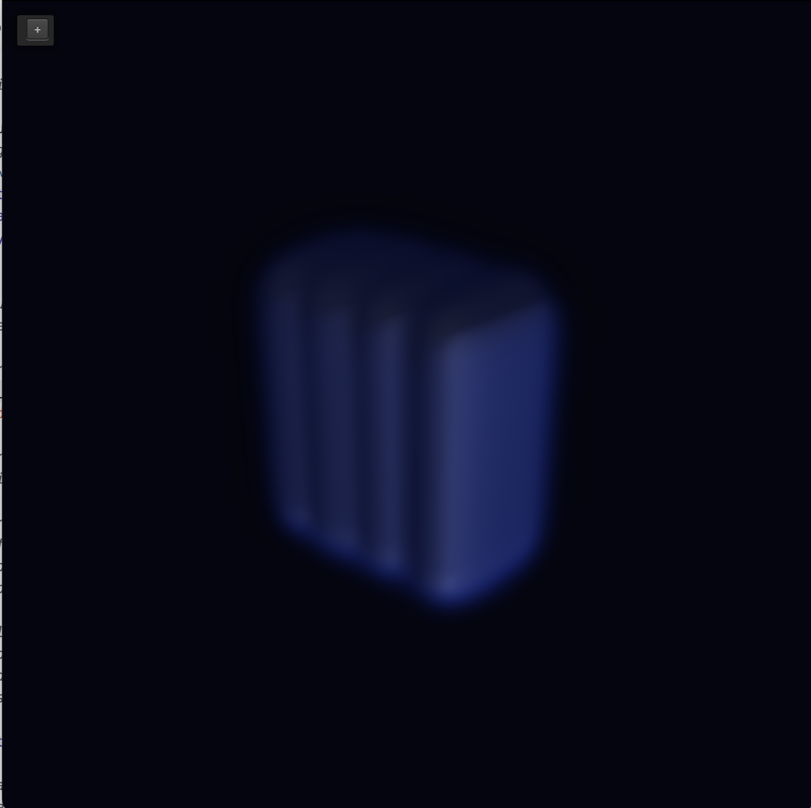
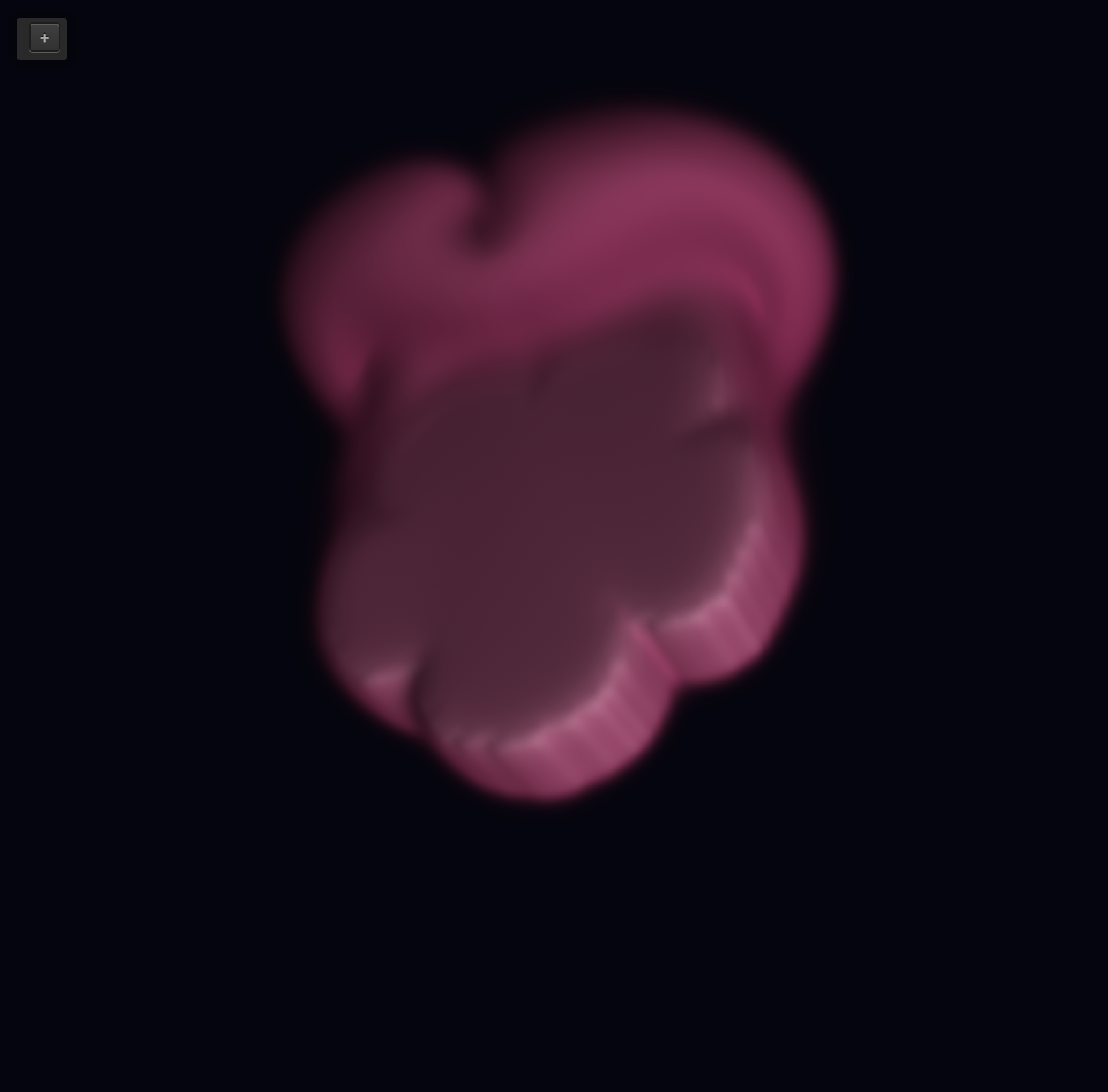
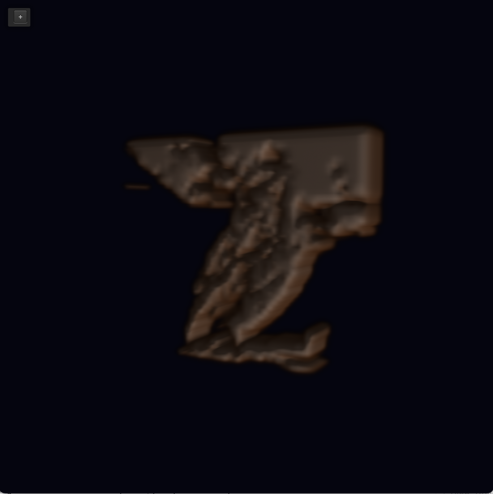
For 3D fluid rendering, we extended the same idea with Stam's stable fluids from 2D simulation, but to a cube of cells. Each cell stores three wind components (x, y, and z) plus smoke density. Every timestep, we update that 3D wind the same way we did in 2D. We blend cells (what does visocity mean in this context), correct the wind so it doesn't falsely bunch up or vanish in each cell, then move the wind/smoke accordingly and correct again. After that, we move the smoke density along the final 3D wind, blur it slightly between neighbors, and fade it with decay. New smoke still comes from emitter cells, which we build from our letter mask like before. We copy the 2D shape into 3D by created a thin layer of depth cells.

This is different from our analytic 3D mode, where the wind is not simulated (it came from a fixed math formula). In fluid 3D, the wind is actually stepped forward on the grid each frame, closer to the physical picture aka a bit more physical accurate. It only changes how density is being used, and the rest of the processes are the same.

Runtime comparison

3D fluid rendering is the heaviest process. Every timestep, it updates three velocity components on an N^3 grid. There are multiple diffuse solves, two projection passes, wind movement of velicty, and then density diffusion and movement. So we are doing multiple full-grid passes over N^3 cells, where you are iterating over the whole 3D grid multiple times per diffuse.
3D analytic rendering is a bit lighter than 3D with Stam's. It still walks through the whole N^3 density grid for wind effect and smoothing, but there is no full 3D velocity solving. Wind is solved via a formula, not stored and iterated like in fluid.
2D fluid rendering is typically lighter than 3D fluid, because the domain is N^2. 3D analytic is still more computationally intensive than 2D, though.

Problems encountered

We had a problem were the smoke was acting like the mouse was just in the top left corner of the screen. The simulation was using positions that were about half as far along as the real cursor. On a Retina Mac, there are two notions of size: the window size in points, where the mouse lives; and the framebuffer size in pixels for Open GL. But the mouse from the GLFW library matches the window size, not the framebuffer. Our code divided the mouse coordinates by a pixel ratio regardless, which shrank them about halfway. To fix it, we got rid of that extra divide, and our cursor moved accurately after that.
Another problem we encountered that we weren't able to resolve was allowing the cursor to move the 3D smoke (via the same logic as 2D). We tried to implement it, but it was very very choppy and delayed. You would move the cursor, and rather than the smoke moving with it, nothing would happen. Sometime later, a bubble-like think would just protrude from the smoke form, and sloppily vanish. It was strange, so we figured that means it's too computationally intensive for a personal computer. Instead, the mouse now just moves the camera in 3D.
Overall, the 3D rendering definitely does not look as smooth as the 2D rendering. It looks stuffy, but this is likely not the product of poor code. Instead its about the CPU/GPU of the computer running it.

Lessons learned

We learned that getting a fluid simulation to look realistic was not only about Navier Stokes math. A lot of the work was in making simulation, rendering, and input all agree on coordinate systems and update timing. We also learned that 2D and 3D versions of the same idea in theory can actually look very different when actually implemented.

2D smoke was much easier to modify and debug than 3D.
Stable-fluids steps/factors are very sensitive to parameter tuning (which we did in the GUI: even the smallest change in the slider caused a great change in the smoke).
There is a distinction between visual quality and physical correctness; they are two separate challenges