In this project, we implemented a ray tracer to render realistic-looking images of scenes with objects and light sources. Ray Tracing is a technique where a computer program uses basic mathematical models of geometric optics to follow the paths of light rays and see how they would be seen by a viewer at a fixed position in the scene. There were 5 parts of this project. In Part 1 we generated camera rays and calculated ray-scene intersections with the camera rays and the scene intersections using the tools of vector analysis. In Part 2 we accelerated ray-scene interesection using a Bounding Volume Hierarcy, which allowed logarithmic-time lookup of our scene objects and thus sped up the rendering process. In Part 3, we traced the light rays that would hit the camera through zero-bounce or one-bounce paths; this required implementing the diffuse BSDF to model the bounce of surfaces, and importance sampling of the lights to speed up how many samples we needed to take to get accurate renderings. In part 4 we solved the global illumination problem, which aimed to model all possible bounces of light through the scene, with exponential decay in intensity at each bounce. While it was infeasible to try to trace infinitely many bounces of light, we could use the Russian Roulette technique of probabilistically killing a ray to get an unbiased estimate of the up-to-infinite bounces of light. In part 5, we sped up our implementation of global illumination using adaptive sampling, which calculates a 95% confidence interval of our perceived intensity every few samples, and if the variance is small, we assume the light intensity has converged and avoid additional sampling.
The main challenges we faced in implementing this project were debugging our ray tracing algorithm for one or more bounces of light in a scene. We had to make sure to be careful with which intersections the ray encountered, and set everything up correctly when making the recursive call. Also, when importance sampling the lights, we needed to make sure that if a reflected camera ray actually hit something else before hitting the light, it shouldn't get the luminance from the light. While it was easy to grasp many of these concepts at a high level, we neeeded to make sure to consider all the edge cases and implementation details when turning the ideas into code.
Part 1: Ray Generation and Intersection
To generate camera rays, we need to construct vectors between the points of the camera origin to the coordinate positions on the image. We have to convert these rays from the camera space coordinates to the world coordinates, then trace these rays through our 3D scenes and identify intersections with objects. To choose which parts of a pixel to trace a ray through, we sample positions at random.
Once we had generated the camera rays through the pixel samples, we traced these rays through our scene and determined if they collided with any objects. Specifically, we needed to implement the equations for the ray-triangle intersection and the ray-sphere intersection. While the equations for ray-sphere intersection are quite easy to derive from the equation of a sphere, the ray-triangle intersection proved to be a bit trickier.
The triangle intersection algorithm was similar to the algorithm that was introduced in discussion section. We first identify a point on a triangle in terms of its Barycentric coordinates and set up a system of equations for [t, b1, b2], where t is the varying parameter of the ray and (1 - b1 - b2, b1, b2) are the barycentric coordinates of an aribtrary point in the triangle. We'd get 3 equations (one from each of the x, y, and z coordinates of the point of intersection) and thus can solve the simultaneous equations using matrix inversion (provided that the matrix is invertible—if not, this means the ray misses the plane entirely). Using the values we get for (t, b1, b2), we can check that (1 - b1 - b2, b1, b2) all lie within the [0, 1] range (ie. the point is actually on the triangle) and that our t > 0 (ie. we are on positive side of the ray) to determine if the ray hits the triangle, and if so we know where.
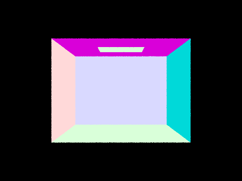
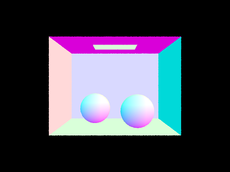
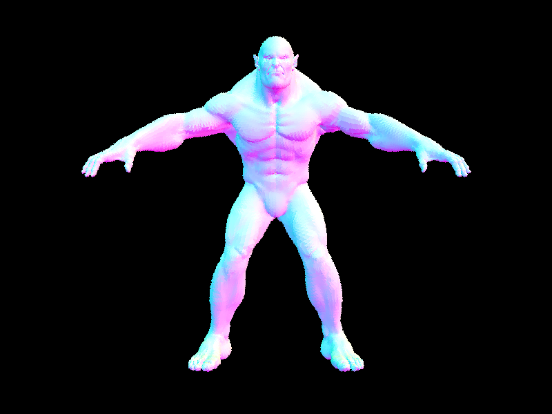
Sample images of ray tracing and intersections
|
|
|
Part 2: Bounding Volume Hierarchy
A Bounding Volume Hierarchy (BVH) is a data structure to accelerate ray tracing in scenes, which uses a tree structure of the objects present in the scene in order to facilitate quick lookup based on location. This way, when tracing rays through our scene, we can quickly identify ray-scene intersections based on the positions of the objects rather than have to iterate over all objects in our scene. To construct a BVH of the objects in the scene, our approach was to first choose an axis along which to split, then identify the value along that axis where we split.
We chose to use axis with the largest dimension bounding box as the axis along which to split. Along this axis, we chose the split value based on the average of the centroids of all the objects within that group. Once we had a split point, we partitioned our list of objects into these two groups based on where the object's centroid was relative to the split point. We then recursively call our function to construct the BVH down to the base case where we have just a few objects left (less than max_leaf_size) left in each leaf node.
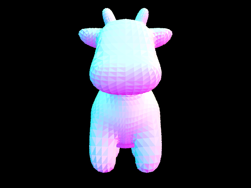
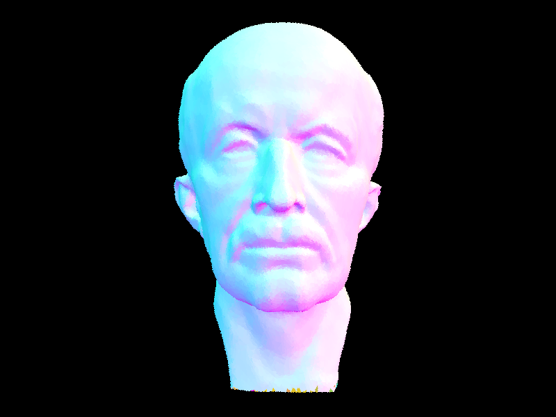
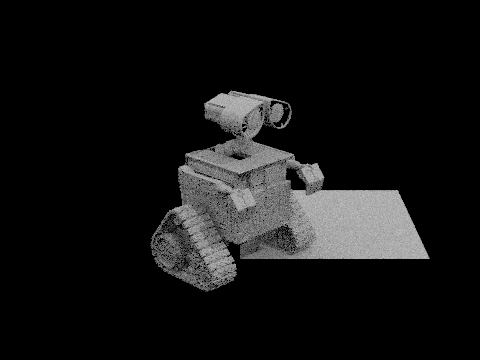
Large scenes only renderable with BVH
Note that the scenes rendered below were infeasible for us to render without the BVH since they have very complex mesh structures which would take prohibitively too long to render. They could only be rended with the BVH acceleration.
|
|
The table below summarizes some of the runtimes of rendering some other complex objects with and without BVH acceleration.
Analysis of BVH optimization
| File Name | Unoptimized intersect | BVH optimized intersect |
| cow.dae Rays traced: 480000 rays | Render time: 96.7616s Avg Intersections per ray: 5856.00 | Render time: 0.8400s Avg Intersections per ray: 29.65 |
| teapot.dae Rays traced: 480000 rays | Render time: 36.1625s Avg Intersections per ray: 2464.00 | Render time: 1.3799s Avg Intersections per ray: 46.17 |
The rendering times with the BVH acceleration were always much faster than the rendering time without using the BVH. This is because without the BVH, any ray-object intersection requires looping through all the possible surfaces in the scene, which is inefficient and costly; it takes O(n) time to find something we want in our scene. With the BVH, however, the average-case runtime to find an object is reduced to O(log(n)) because the tree structure allows fast lookups.
Part 3: Direct Illumination
The direct illumination function considers rays of light that take zero or one bounces to hit the camera. For zero-bounce, we just need to trace the a ray from the camera to light sources and consider the amount of light emitted from the source.
For one-bounce, we need to trace the camera ray through a pixel to its first intersection point with an object in the scene, then estimate the total illuminance at that point from light sources in the scene. Since computing incident surface illuminance requires integrating the incoming luminance of light coming from all directions over the hemisphere, we need to numerically evaluate this integral using Monte Carlo Integration, which takes sample directions and calculates the radiance of rays coming from those directions hitting the surface.
There were two main approaches to performing this Monte Carlo integration. One approach used uniform hemisphere sampling, ie. we choose a point at random from the hemisphere and consider the contribution of a light ray coming from that direction. However, if there are only a few light sources, this approach may generate many rays that contribute little to the actual integral because the reflected camera ray does not end up hitting a light source. Thus, an improvement to get more "useful" samples is to perform importance sampling, where we sample the light sources directly.
Our implementation of the direct lighting function with uniform hemisphere sampling first constructs a camera ray and identifies the first hit point. Then we take num_samples sample directions and trace them to their next intersection. If the next intersection is a light source, we add the radiance contribution to our estimate (normalized by the pdf of that direction vector) and divide by num_samples once completed.
For the direct lighting function with importance sampling, we again trace camera rays to the first intersection point, but from there rather than take num_samples samples, we iterate over the light sources in the scene directly. For point light sources, we add their radiance contributions (normalized by the pdf). For area light sources, we take ns_area_light samples in directions that hit the light and add their radiance contributions (normalized by both the pdf of the direction and the ns_area_light). In this case, we needed to check that we didn't hit another object first as we travel in the direction of the ray, since then the other object would occlude the light source.
For ray tracing, we needed to make sure to start our ray's t parameter at a small "epsilon" parameter to avoid hitting our own surface due to floating point precision errors, and also keep a buffer of epsilon before the light source to check if there were any other objects in the scene.
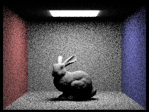
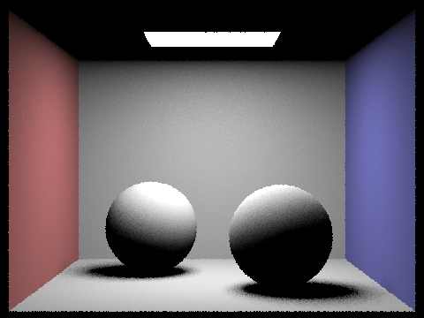
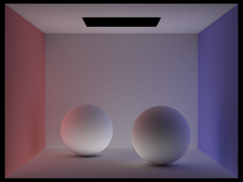
Examples of direct illumination with and without importance sampling
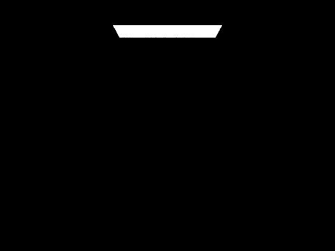
| zero bounce |

|
|
| one bounce with hemisphere sampling |
|
|
| one bounce with importance sampling |
|

|
Uniform hemisphere sampling requires a much greater number of samples to estimate the true contribution of lights, since it may end up sampling many directions which never hit the lights. Importance sampling, on the other hand, samples the light sources directly because they are the only things that contribute non-zero values to the integral. This is why with the same number samples, importance sampling renders much more accurate and less grainy results compared to uniform hemisphere sampling which ends up getting lots of samples that we don't care about (since their contribution is 0). Note that because a given sample's contribution to the integral is weighted by the reciprocal of probability density function in Monte Carlo integration, both uniform hemisphere sampling and importance sampling get approximations that are consistent (ie. approximate the true value).
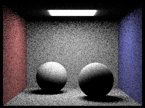
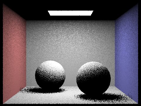
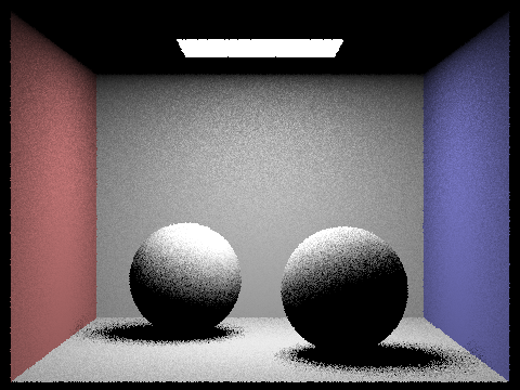
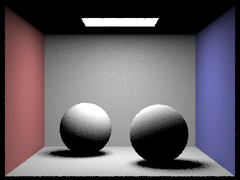
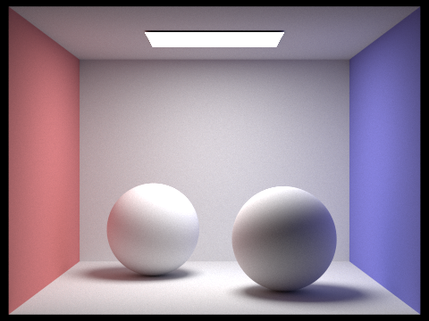
The images below show the scenes rendered with different numbers of light rays cast, using 1 sample per pixel and importance sampling of the lights.
|
|
|
|
As we take more samples of the number of light rays cast, we notice that the noise levels decrease. This is particularly evident in the soft shadow regions under the sphere. This makes sense, as when we have more samples we get a better estimate of the true value of our integral and thus have less noisy images.
Part 4: Global Illumination
The global illumination problem aims to trace all possible bounces of light (even if more than 0 or 1) that eventually hit the camera. This turns out to be an converging infinite series sum, since some light is disappated at each bounce but there can be an arbitrarily large number of bounces that a light ray encounters before making it to the camera. Our implementation considers the zero-bounce radiance (directly from light source) and at least bounce radiance. The function for at least one bounce radiance is recursive, since it considers the contribution from one bounce directly off the first intersection point, and at least one bounce radiance from other points that eventually hit the first intersection point. Since the sum total would have infinitely many terms, we terminate when we have traced a ray through more than max_ray_depth bounces. We also implemented the Russian Roulette technique to terminate rays, where at each bounce, each ray continues with some probability rr_prob and is terminated (killed) otherwise. We add up the contributions from the one bounce-radiance at a point and the result of the recursive call (contributions of later bounces) to get a final value of the illuminance at a given point.
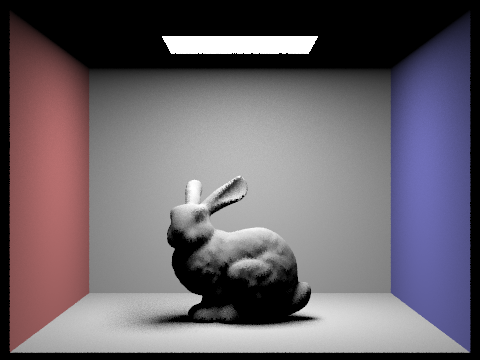
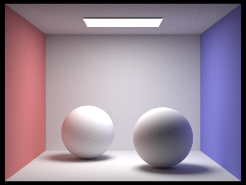
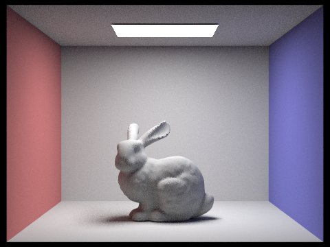
Scenes with global illumination
Below are some scenes rendered with global illumination.

|
|
|
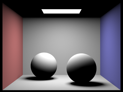
Direct vs Indirect illumination
The images below show the contributions of the direct illumination (zero and one-bounce) and indirect rays of light (more than 1 bounce).
|
|
|
Ray depth cutoff
The images below show rendered views with various values for max_ray_depth (m). This refers to the maximum number of bounces a ray will trace.
|

|
|

|

|
Samples per pixel
The images below show the rendered views with different number of samples per pixel (s). As you can see, having more samples per pixel leads to much higher quality, less grainy renderings.
|
|
|
|
|
|
|
|
Part 5: Adaptive Sampling
Adaptive Sampling is a technique to speed up renderings of images. We first estimate the mean and standard deviation of the luminance along a camera ray using the samples taken so far. Using the estimate of standard deviation, if 2 standard deviations (corresponding to a 95% confidence interval) is below a certain threshold, then we don't need any more samples and can conclude that the illuminance has converged. Our code is able to quickly estimate the mean and SD of the samples taken so far by keeping track of the sum and sum of squares of the sample illuminances taken so far. From there, we use the simple formulas provided in the project specification to get the estimates.
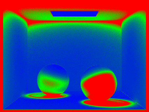
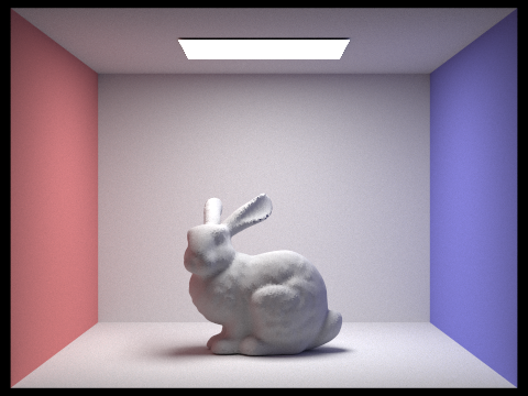
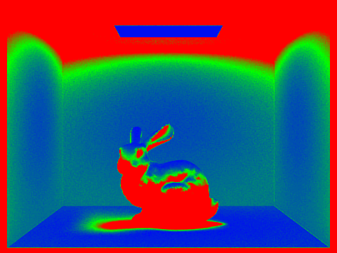
Variable sample rate
The images below shows some renderings of scenes generated with adaptive sampling, as well as heatmaps of the sampling rates per pixel. Red indicates more samples taken, while blue means less samples taken. All of these were rendered with 1 sample per light and a max ray depth of 5.
|
|
|
|
Final Thoughts
As a partner project, this was a very collaborative experience and we needed to rely on one another to get the project working. Both of us met up in-person and on Zoom most of the times that we worked on the project. Pair programming proved to be an effective way for us to catch bugs early and solve problems as they arose. Towards the end, Rishi focused on debugging many minor issues with our implementations and generating high-quality images while Saagar focused on completing the writeup.