CS 184: Spring 2022
Sam Ellgass and Nima Rezaeian
In Project 1: Rasterizer, we implemented the entire rasterization pipeline for SVG files with a number of customizations to allow us to experiment with different techniques of supersampling and pixel/texel interpolation. By creating methods that work with generality on triangles, this allowed us to experiment with different combinations of sampling and interpolation methods on the same set of images to easily compare and contrast results.
The build that we've implemented is able to render any combination of points, lines, and triangles, and interpolate those triangles with color or texture at several levels of supersampling, interpolation, and with the use of mipmaps. One of my most significant takeaways from this project is just how important it is to understand how a texture has been modified before displaying it on screen. The use of mipmaps as well as different strategies for triangle interpolation make it obvious that a good render must take into account transformations and variations from a static texture.
In this task, we implemented the ability to display, color, and render triangles. First, we calculated whether or not the winding order of a triangle was consistently counterclockwise. After putting the vertices in the correct order, we used a bounding box from min(vertices.x), min(vertices.y) to max(vertices.x), max(vertices.y) in order to make sure that we only did as many point-in-triangle calculations as necessary. Then, we iterated over all of the possible pixels within the bounding box, and if they fell within the triangle, put the triangle's color in the sample buffer. Finally, the sample buffer was iterated over to be resolved to the frame buffer and displayed.
Since we made sure to only assess pixels within the bounding box, our algorithm is relatively efficient. The main challenge we faced in implementing simple triangle rasterization was assessing winding order. After realizing that a consistent winding order was crucial to accurately using the point-in-triangle test, we made sure to reorder the vertices consistently, and our method was able to work in general. We also had to make sure to test points at the "<=" edge boundary, since there was no asymptotic harm and it made sure that even with slight rounding error, we rasterized the edges of the triangle.
In this task, we expanded the functionality of our triangle rasterization to allow for supersampling. We used the same algorithm as in task 1, but instead of iterating through the entire bounding box by pixel, we iterated through the entire bounding box using a step size of square_root(sample_rate). We also expanded the sample buffer to accommodate a factor of sample_rate more samples. Then, in our resolution to the frame buffer, we made sure to consider all of the samples that corresponded to one pixel's worth of data before resolving that pixel to the frame buffer. The main change that this caused was that our resolution to frame buffer, rasterization of lines, and buffer operations had to be updated to account for this.
Supersampling resulted in antialiasing for triangles by averaging across different samples within each individual pixel, while still preserving the form of the image and without changing the fidelity of lines and points. This allowed jaggies and other artifacts at points of high frequency to be smoothed and appear more gradual. The most challenging part of this task was trying to understand edge case behavior with sampling. In the end, we realized the importance of maintaining only integers within our for loops and only using fractions in local operations to avoid cascading floating point errors. Additionally, we had to carefully consider our new sample buffer in order to preserve "fill_pixel" for lines and points, and having consistent loop structure greatly helped this in the end.


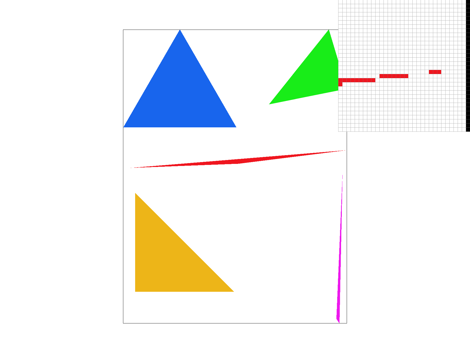
Above, the effects of supersampling on an area of high frequency are shown with sample_rate = 1, 4, and 16. Supersampling can be seen to antialias otherwise harsh artifacts in areas of high frequency change.
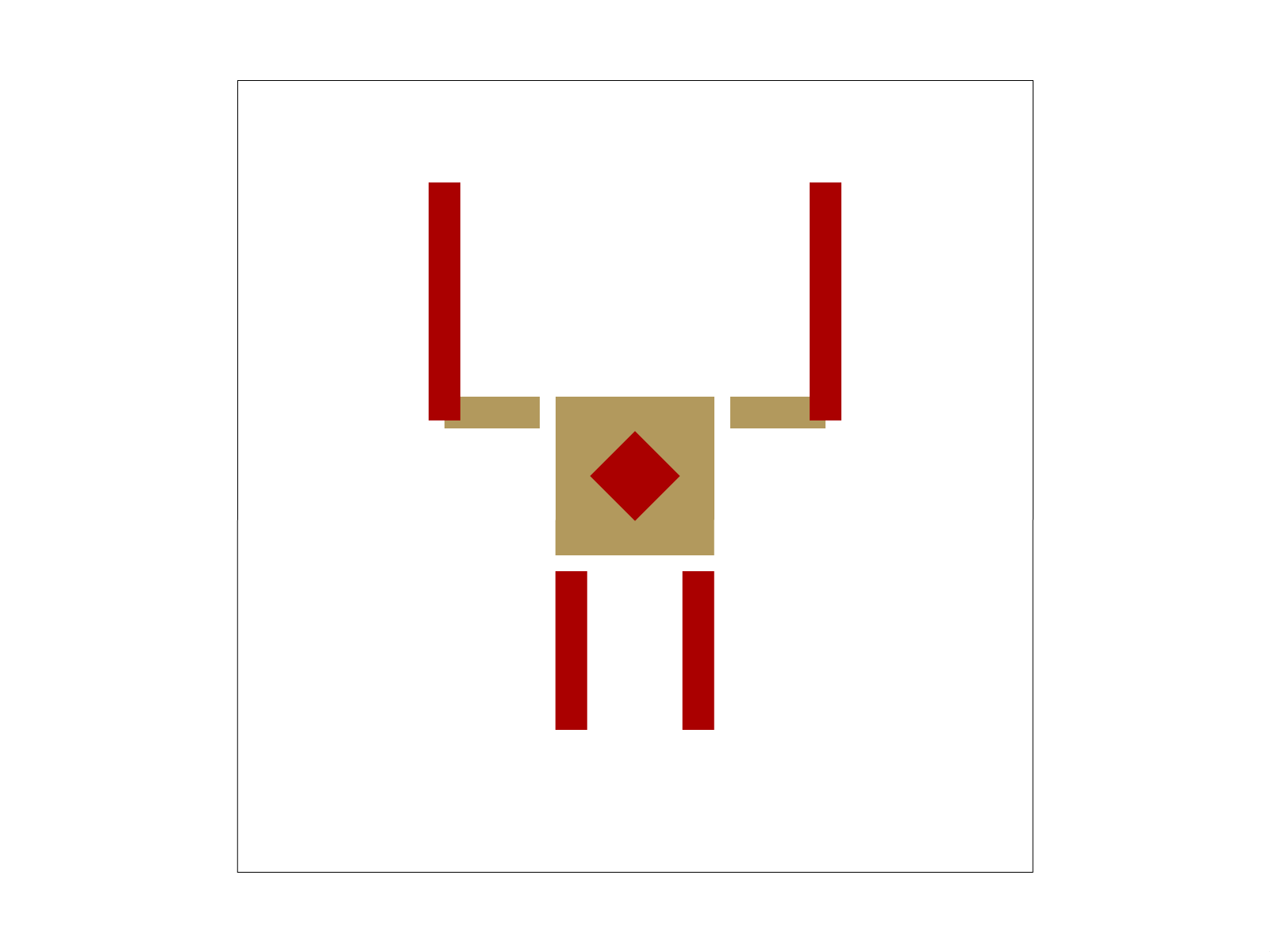
Using homogeneous coordinates and GL's Matrix3x3, we implemented rotate, scale, and translate transforms that could easily be applied to SVG elements. Our variant of cubeman.svg is called "Average 49ers Fan", and depicts a San Francisco 49er's fan in the Football "field goal" position in the trademark 49er's colors. By lengthening and transforming the arms into field goal position, shortening and connecting the legs to give him a smaller stature, and comically lowering his head into his lap, our cubeman is in a completely different state.
In this task, we implemented barycentric triangle coordinates in order to specify points in a triangle by relating an interior point to the three sides of the triangle. This is achieved by proportional distances to each side. Below, see triangle ABC where vertex A is green, B is blue, and C is red. Then, any point can be defined by its distance to vertex A relative to side BC, vertex B relative to side AC, and vertex C relative to side AB. These proportions then define closeness to each vertex, and thus a point much closer to A than BC will have a high alpha value and be colored more green, and so on.

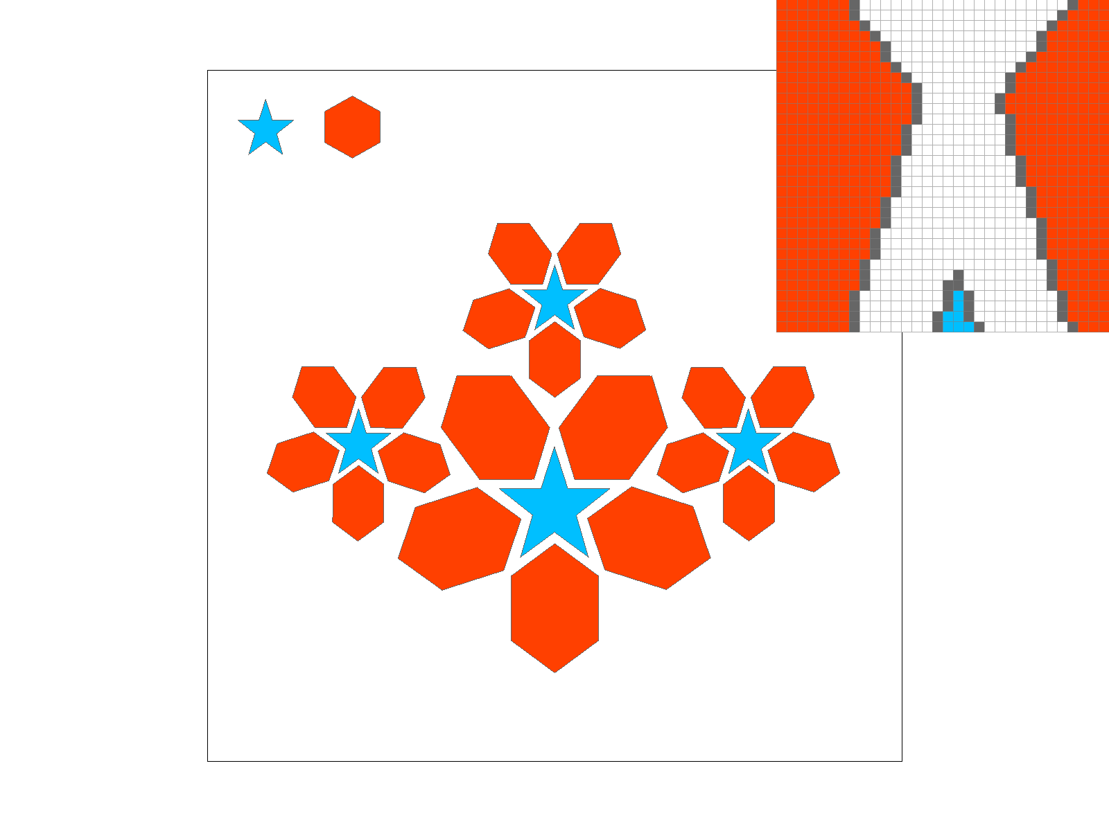
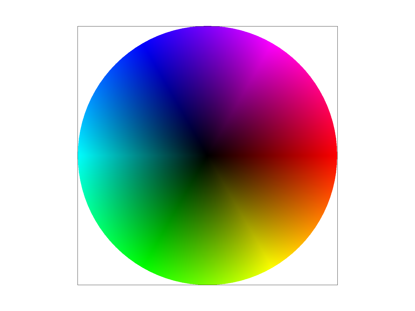
Below, svg/basic/test7.svg (color wheel) is shown rendered with our methods. No changes to the color gradient were made, so the image below is as intended.
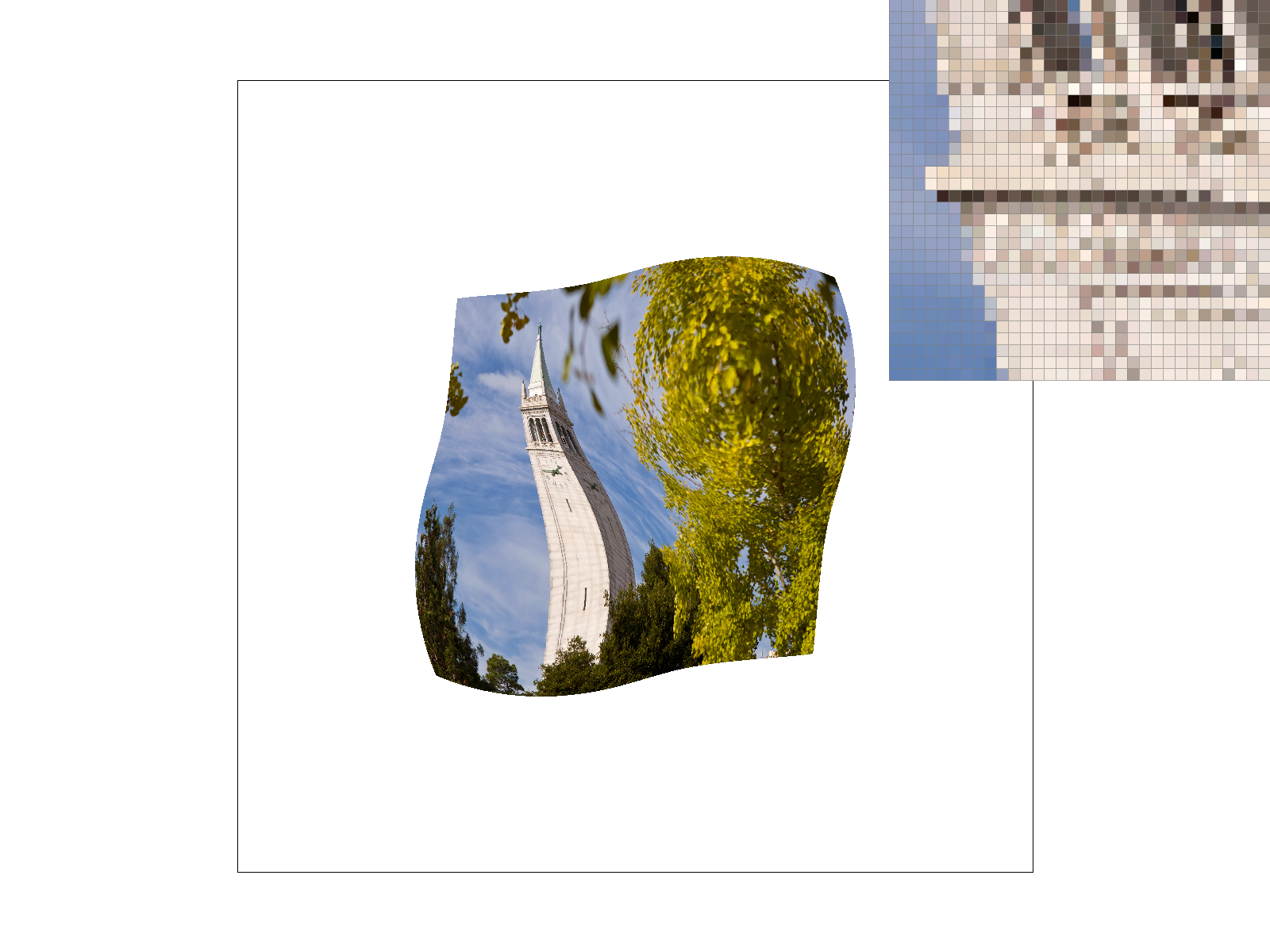
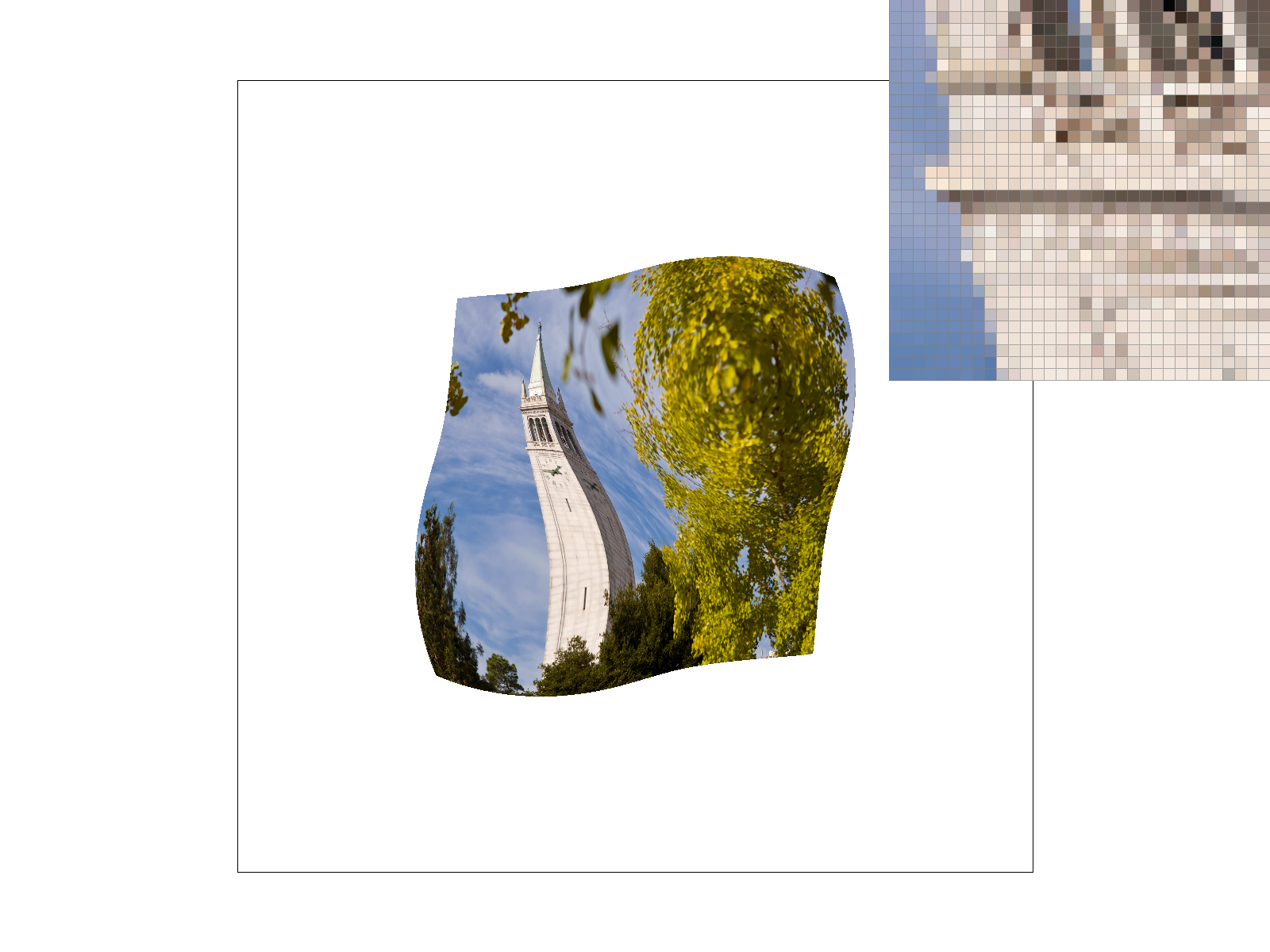
In this task, we implemented texture mapping with two methods for pixel sampling: nearest and bilinear. Pixel sampling is using the colors from a texture to map some part of that texture appropriately onto a polygon in screen space. Nearest sampling simply finds the texel that is closest to the corresponding coordinate in the polygon, while bilinear takes into account distance from the four nearest texels, and combines them using distance to the true location as weights.
Below, see an example of bilinear sampling clearly creating a higher quality image than nearest sampling on the following transformed texture of the campanile. With nearest (left), the frequency of change at the base of the campanile creates noticeable artifacts that are somewhat softened by bilinear sampling. However, when supersampling with sample_rate = 16, this effect becomes much less noticeable! This makes sense, since as the sample_rate increases, the "nearest" sample starts to approximate the bilinear sample, and though without linear interpolation's weights, the weights will decrease as sample rate increases, making the two more similar at higher sample rates.


In this task, we implemented texture mapping using level sampling methods to inform which mipmap level was used. Level sampling uses some information from screen space to decide what fidelity that a given texture should be sampled at. Trilinear interpolation (bilinear level sampling) uses a weighted combination of the two nearest depth levels, where depth is calculated by looking at the highest frequency partial derivative from screen space with respect to texel coordinates. P_NEAREST uses the same depth calculation, but simply rounds that to decide which mipmap level to sample from. P_ZERO simply always returns a level of 0, the highest resolution image. In our implementation, we perturbed our x,y point in screen space and did barycentric triangle interpolation using those perturbed points to find the rate of change, and then used the corresponding level of the mipmap to sample texels for our image.
P_LINEAR is the most accurate method and the costliest, with smoothing to overcome the sharp changes of P_NEAREST - as well as generally also the highest antialiasing - but a runtime that takes twice as long. P_NEAREST, in turn, is more accurate and costly than P_ZERO, but offers a significant improvement in cases of minification of a texture. P_ZERO offers no antialiasing, but is immediate, requiring no calculation.
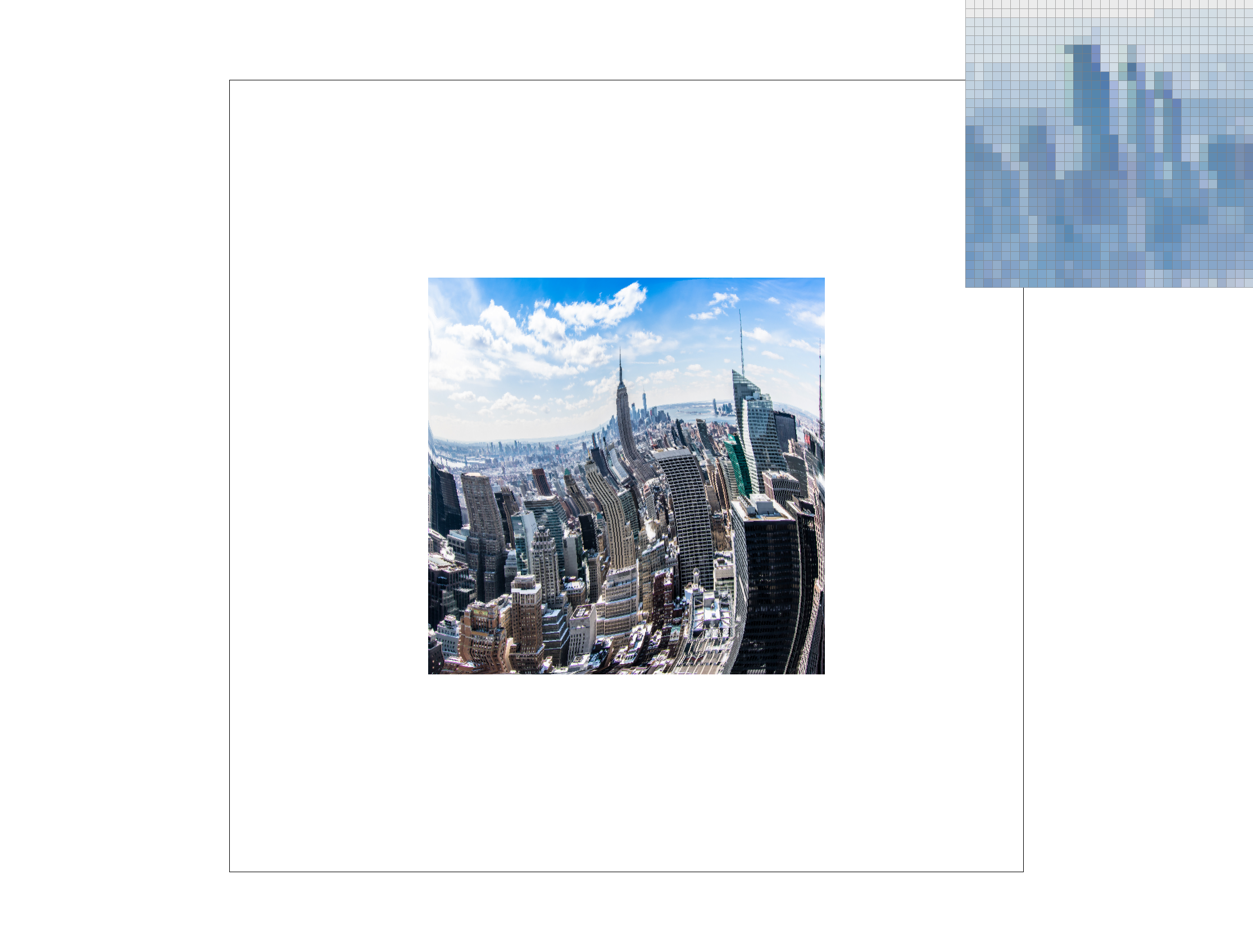
Below is a PNG of a Landscape taken in New York City (credit Lukas Kloeppel) rendered as a texture. For this image, it's clear that using mipmap levels is important - both with the transformation of the polygon and with the incredibly high resolution (and high frequency) of the buildings in the distance. Thus, when we use a level sampling method of L_NEAREST, the fidelity of the image improves greatly. Interestingly, I personally like P_NEAREST as a pixel sampling method in this case over P_LINEAR, as we think it's important to have some image quality in the distance.


We thoroughly enjoyed this project. Getting to understand the tradeoffs between different antialising techniques by actually implementing and understanding their performance (on my CPU) was very informative. The freedom that transforms and texture mappings offer was my favorite part of this project, and something we want to explore more in the future.
Most of our major challenges stemmed from misunderstandings with how best to handle a very large volume of cases consistently (edge cases for triangles, winding order, precision errors due to poorly constructed loops), and thus we can confidently say that we have a better understanding of how to handle enormous, precise data stuctures after this project.