CS184 Project 1: Rasterizer

By Team Lucies (Lucy Lou and Lucy Wan)

Overview

In this project, we rasterized triangles from three given vertice points and different colors. We started off simple with sampling per pixel, then moved on to implement supersampling and texture filtering on pixels and mipmap levels. We also wrote functions to support transforms and color gradients. It was interesting seeing the drastic difference going from single pixel sampling to texture filtering, and being able to switch between the two easily. It was also interesting to realize that color gradients can be formed from triangles with interpolation of the colors.

Task 1: Drawing Single-Color Triangles

In this first task, we are given the 3 points of the triangle. We found the minimum X, maximum X, minimum Y, and maximum Y values from these points and took the floor of the minimums and the ceiling of the maximums so they were rounded to integers that could form a rectangle we can loop through. We then had a double for loop, starting from minX+0.5 and minY+0.5 and incrementing by 1 pixel because we wanted to check if the center of the coordinate was in the triangle. Inside that double for loop we called the function inside from triangulation.cpp to check if the current x and y coordinate our loop was on was inside the triangle. If it was, we called fill_pixel() with those x y values and the given color. Lastly, we updated the inside function in triangulation.cpp to support different vertex input orderings by including that if all the cross product signs were negative, the point is inside the triangle (before only the case where all the cross product signs were positive was accounted for).

We used a bounding box for our algorithm, but even if we hadn’t used a bounding box, it would have been no worse in terms of image quality since both methods lead to the same image. Bounding box only reduces redundancy in terms of calculations which in turn makes our application faster.

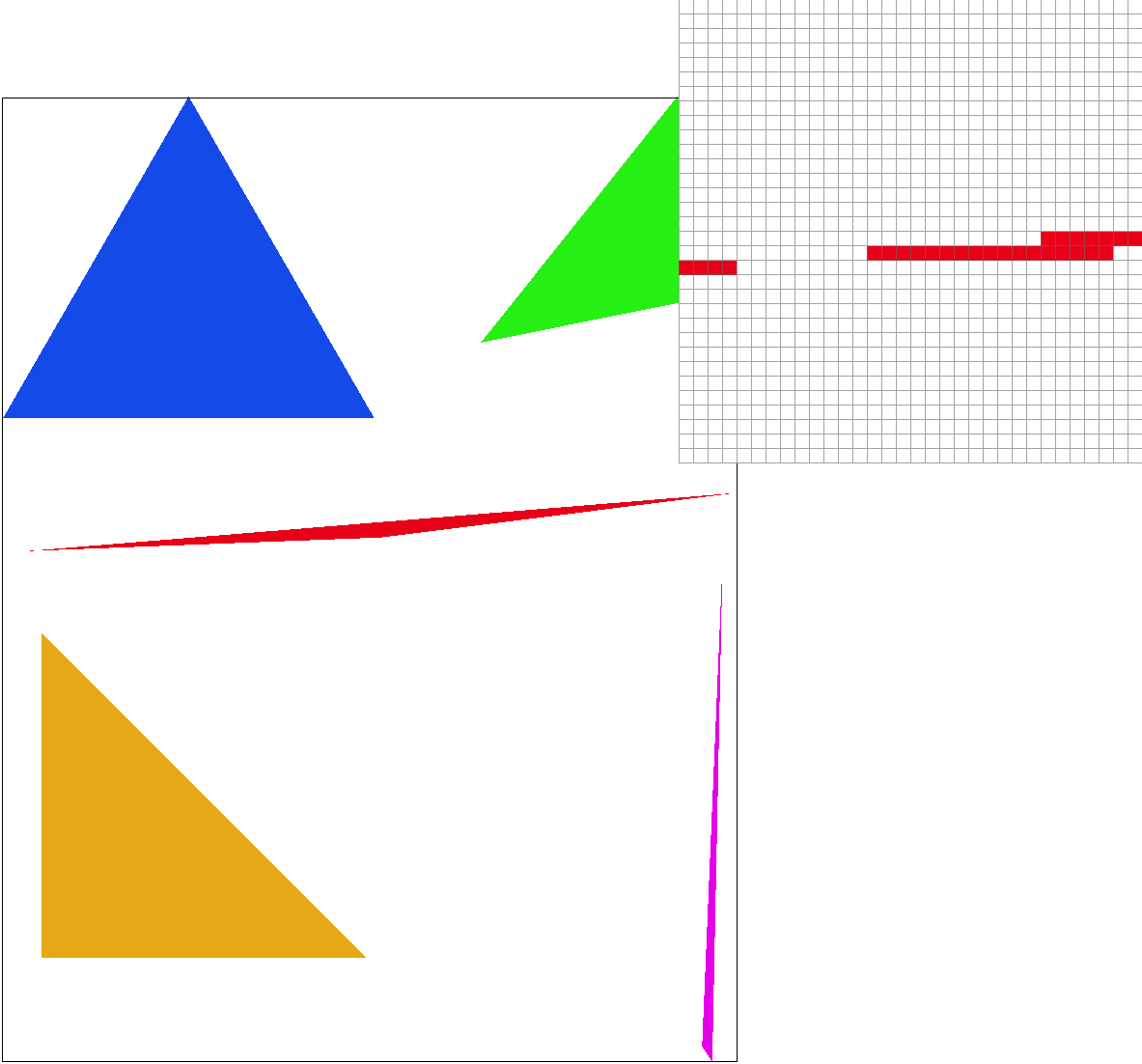
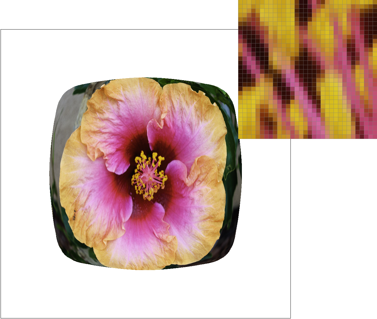
Here is an example of rasterized triangles. Since we are sampling at 1 pixel, the boundaries are very sharp with jaggies. In fact, as shown with the pixel inspector, on the very skinny red triangle, the tip isn’t even connected.

Task 2: Antialiasing by Supersampling

To implement supersampling, similarly to task 1, we used the same two data structures as Task 1, the sample buffer (for storing sampled values) and the frame buffer (for storing pixels to be displayed). We also loop through the triangle bounding box to account for every point in the triangle. However,now we also add a double for loop to loop through the subsamples within each pixel. We start at an offset of ½*sqrt(sample_rate) and increment by 1/sqrt(sample_rate) both in the x and y directions to iterate through each subsample. We check if the area sampled is inside the triangle and if so we store the color value in our sample buffer at the correct index, which we calculate by using a counter variable. Our sample buffer is the size of the screen multiplied by our sample rate to account for the extra samples for each pixel. After all the values are stored in the sample buffer, we resolve these values to the framebuffer by taking the averages of the colors we get from each pixel and storing that value in its respective location within the frame buffer. Since the frame buffer stores colors differently from the sample buffer, we had to remember to convert between Color objects and RGB channels in this step. Lastly, we updated our fill_pixel() function to account for the increased sample buffer size by filling in sample_rate amount of values within the sample buffer per pixel (instead of one value per pixel as in Task 1).

Super sampling is useful because it antialiases by decreasing the amount of sharp jaggies found in images. It creates smoother edges by averaging multiple values within a pixel to make the image more blurred rather than sharp. For example, zooming in on non-supersampled triangles with the edges that go diagonally, there is a staircase effect. The same benefits triangles that are very skinny.

For modifications in the rasterization pipeline, as stated above, we modified the sample buffer to account for the sample rate, added a double for loop within our rasterizing function in order to get to each subsample, and averaged the subsamples to get our frame buffer.

We used supersampling to antialias our triangles to blend the edges and the background together creating a smoothing effect.

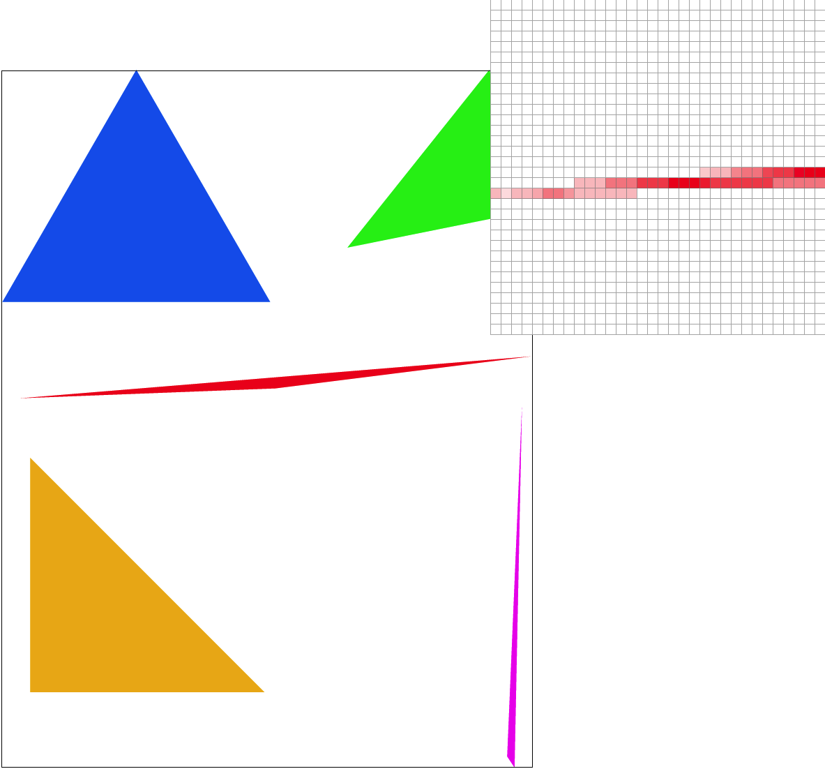
Here is the pixel inspector at the same skinny triangle point. At sample rate 1, each pixel is the same color resulting in jagged edges and an unconnected tip. Increasing the sample rate to 4 already significantly improves the quality. There’s no more unconnected tip and the jaggies are less pronounced; however, it has also slightly cut off the tip by a few pixels. At sample rate 9, we see the full length of the triangle and the point is noticeably smoother, and by sample rate 16 the edges are straighter. These results are observed since supersampling reduces aliasing by having a smoothing effect through blurring jaggies.

Task 3: Transforms

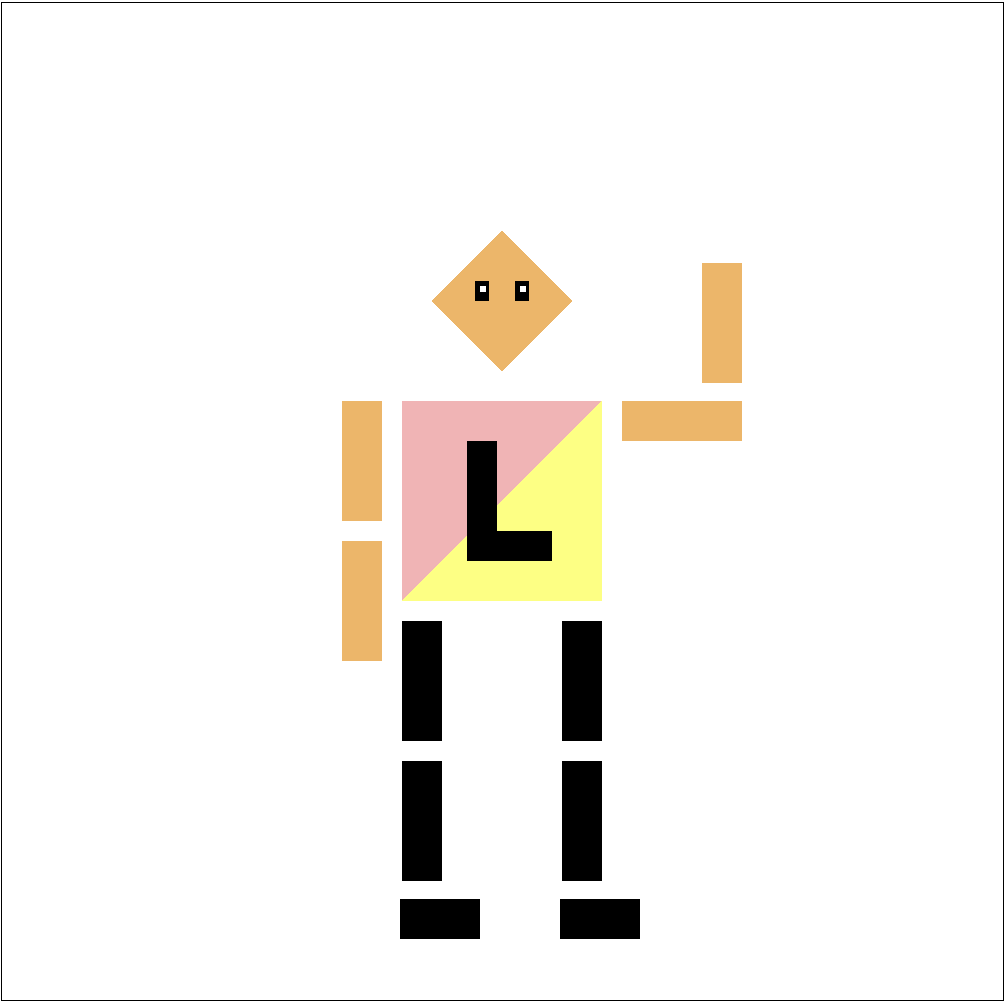
This is Lucy Robot. Both my name and my partner’s name is Lucy, thus the L on the shirt. The shirt is also half baby pink, my favorite color, and half yellow, my partner’s favorite color. Black or white pants go with everything, but since the background was white I went with black. I also added eyes because eyes are the windows to the soul, shoes so she’s not barefoot, moved the left arm down because that’s tiring to have it up, and made the right arm wave because she’s friendly.

Task 4: Barycentric Coordinates

Barycentric coordinates are the distance proportions a point is from each vertex of a shape. As a result they add up to 1. They give us ratios of how much of the values at each vertex to use to interpolate each value within the shape.

In the case of Task 4, our barycentric coordinates are α, β, and γ where V = αVA + βVB + γVC and VA, VB, and VC are the color values of the 3 triangle vertices and V is the value of the point which we are finding the resulting interpolated color.

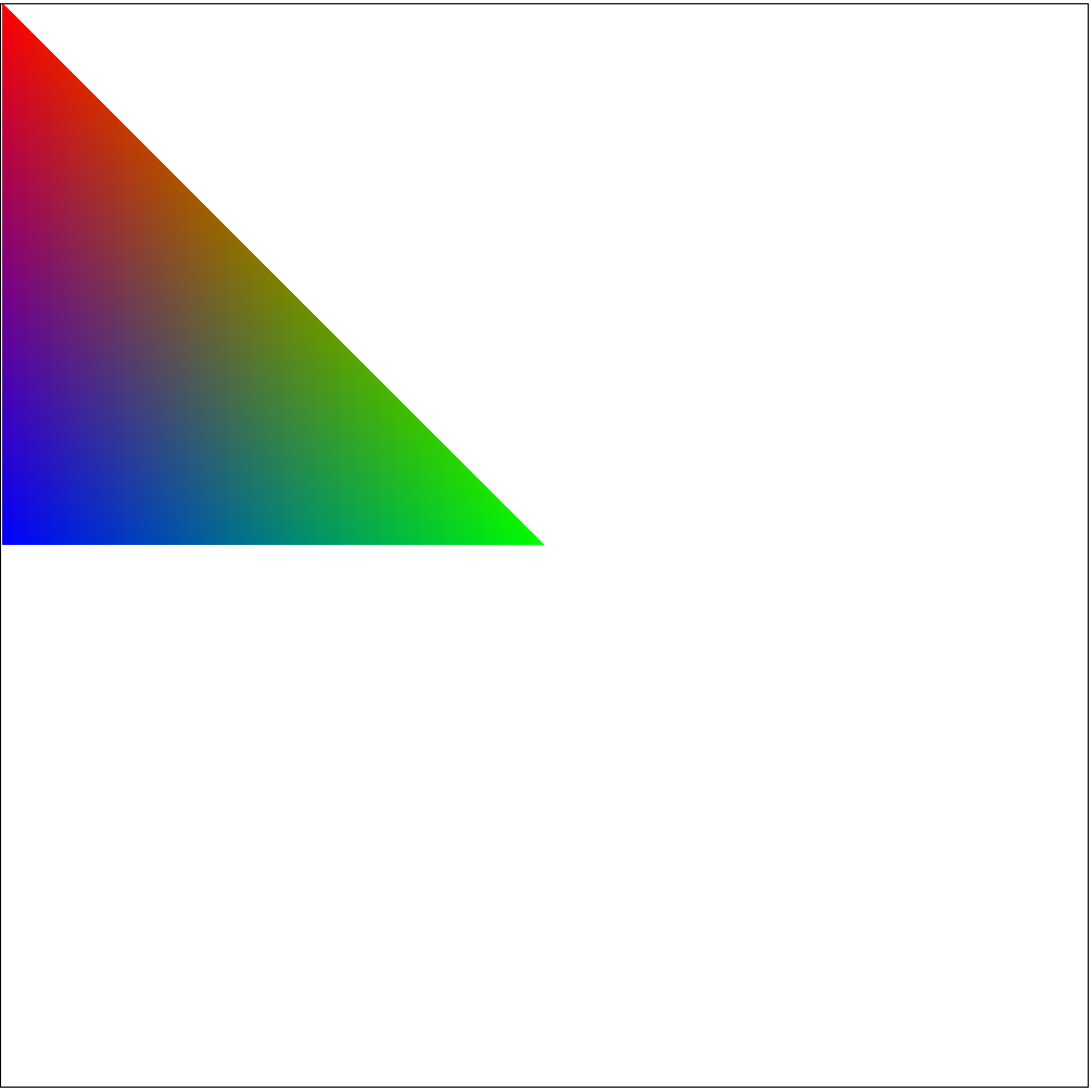
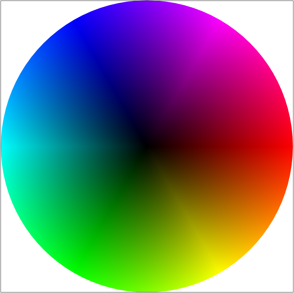
This results in a smoothly blended triangle with each pixel assigned a different color. For example, in the image below we have a triangle interpolated with red, blue, and green corners.

In terms of implementation, we use a similar rasterization algorithm as in Task 2. However this time, instead of simply filling pixels with a given color, we use V = αVA + βVB + γVC to find out what the color of our current coordinate should be. Though there are many ways to find barycentric coordinates, we used matrix calculations since to us it made the code look cleaner. Specifically we multiplied the inverse of a 3x3 matrix [x0, x1, x2, y0, y1, y2, 1, 1, 1] with [x, y, 1] (where (x, y) is the current coordinate we’re looking at)to produce [α, β, γ]. This allowed us to create a color wheel.

Task 5: "Pixel sampling" for Texture Mapping

Pixel sampling is representing a spot in a real life image as a pixel. Nearest sampling takes the nearest pixel to the point we want to sample, so we round the x and y values to get to the nearest pixel. Bilinear sampling uses interpolation of the four pixels adjacent to the point we want to sample. It does this by first interpolating horizontally between the top two points and the bottom two points then vertically with the resulting two points.

To implement pixel sampling to perform texture mapping, we first calculate the (u, v) value of a texture map from the corresponding (x, y) value from the approach in Task 2. We get from (x, y) to (u, v) by finding the barycentric coordinates of (x, y) and applying them to the vertices of the texture map to find (u, v). We then use the inputted pixel sampling method to get the color value at (u, v) using the processes described above.

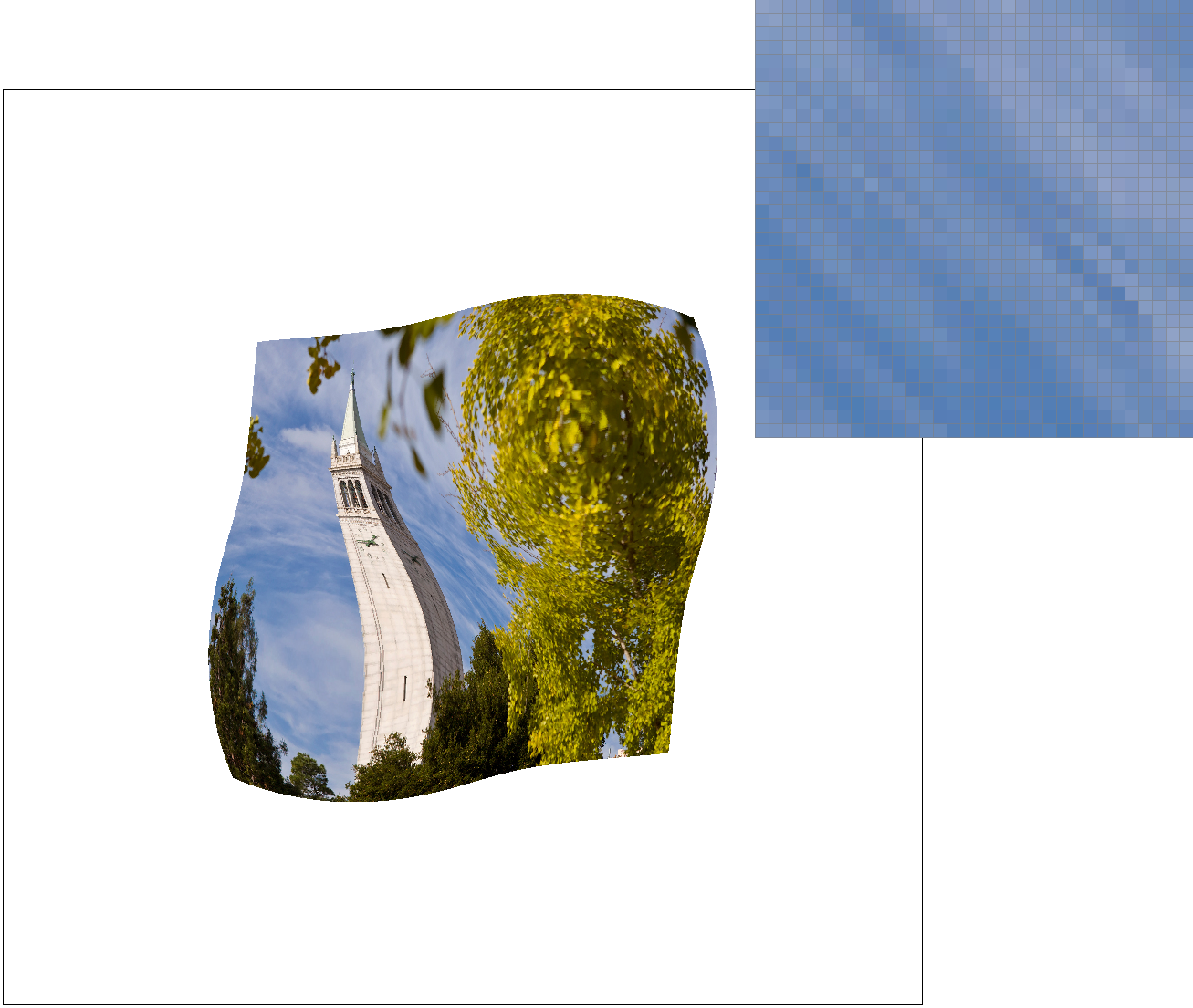
This is an image of the Campanile with the pixel inspector on the windows. Nearest at sample rate 1, has very blocky pixels. By sample rate 16, it’s significantly smoother. With bilinear sampling, even at sample rate 1, produces a better quality, smoother image than nearest at sample rate 1. With both bilinear sampling and supersampling at 16 samples per pixel, we get the smoothest result. The individual pixels are a lot more blended and although the image looks “fuzzier” zoomed in, it looks better at the normal size with less aliasing.

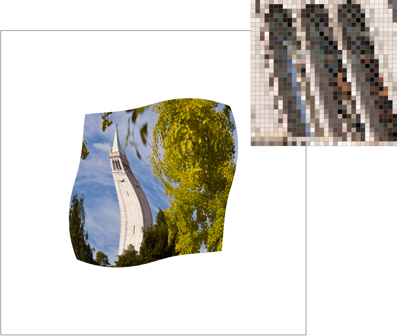
In general, bilinear sampling will make a large difference on images with small details in contrasting colors. A bilinear sampled image will look similar to a nearest sampled one in areas of similar color, for example the sky. This is because bilinear sampling blends multiple adjacent pixels into our sampling.

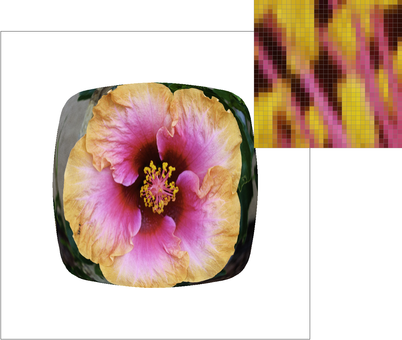
Task 6: "Level sampling" with Mipmaps for Texture Mapping

Level sampling is sampling from different minimap levels depending on how the x and y values adjacent to a point change on the corresponding texture map. The purpose of level sampling is to make an image more realistic by having pixels that represent parts of the image further back to be more blurred. We implemented level sampling by calculating the barycentric coordinates of (x, y), (x, y+1), and (x+1, y) and find their corresponding coordinates on the texture map. We used these values to find our difference vectors du/dx and dv/dy, which we then use to find the level as a float using the equations to find the level as shown in lecture. If our level sampling method is “nearest,” we round this value, and if it is “linear,” we interpolate this value with the colors of the two adjacent levels closest to our float.

Compared to the other two ways of antialiasing, level sampling is likely the slowest since in addition to its own code it calls pixel sampling (depending on what sample_rate within supersampling you are comparing it to). It also uses more memory than pixel sampling as it uses a struct to store dx/uv, dy/uv, and uv. Within pixel sampling, bilinear pixel sampling is slightly more costly than nearest pixel sampling since there are many more calculations involved. However, bilinear pixel sampling produces excellent results. Number of samples per pixel is the most straightforward with minimal calculations, but slow performance as it’s “enlarging” the picture multiple times to achieve the antialiasing. All three antialias well, and the choice of which one depends on the picture.

Comparing the combinations of these forms of sampling, we see when both are used together we get the smoothes image, but it may even seem blurry. Level zero and pixel linear looks a little jaggedy still. Level zero with nearest pixel sampling looks similar to linear pixel sampling, but linear is slightly smoother.

https://cal-cs184-student.github.io/sp22-project-webpages-lucylanlou/proj1/index.html