Link to (this) Webpage

Link to Code

Project 3-1 Pathtracer

Overview

We utilized a pathtracing algorithm to implement the core routines of a physically-based renderer. We implemented functionality for ray generation and scene intersection, we accelerated the process by implementing a Bounding Volume Hierarchy data structure, we implemented direct and global illumination, and we finally implemented adaptive sampling to reduce noise in our images.

Part I: Ray Generation and Scene Intersection

Ray generation and primitive intersection

To generate rays we start from normalized image coordinates (x,y). We first must convert the image coordinates into the camera space and then into the world space. Our normalized image space is in the range of (0,0) to (1,1), and our camera space is in the range (-tan(0.5 * hFOV), -tan(0.5 * vFOV)) to (tan(0.5 * hFOV), tan(0.5 * vFOV)). This first transform is a simple linear mapping. Then, we convert the camera space coordinates into world space using the camera’s camera-to-world rotation matrix c2w. Finally, the origin of our ray is the camera’s position p. We have:

  Ray Camera::generate_ray(double x, double y) const {
    Vector3D direction = c2w * Vector3D(tan(radians(hFov / 2)) * (2 * x - 1),
                                        tan(radians(vFov / 2)) * (2 * y - 1),
                                        -1);
    direction.normalize();

    return Ray(pos, direction);
  }

We then use this generate_ray function when we estimate the radiance for pixel samples. For each sample we create a ray, and this ray will later intersect elements in the scene. The code looks as follows (remember that generate_ray takes normalized coordinates):

  Vector3D average_radiance;
  for (int i = 0; i < num_samples; ++i) {
    Vector2D offset = gridSampler->get_sample();
    Ray ray = camera->generate_ray((x + offset.x) / sampleBuffer.w, (y + offset.y) / sampleBuffer.h);
    average_radiance += est_radiance_global_illumination(ray)  / (double) num_samples;
  }

Finally, we intersect primitives. There are two functions we implement for each primitive: has_intersection(const Ray &r) and intersect(const Ray &r, Intersection *i). The first one simple checks if there’s an intersection between the primitive and the input ray. The second also reports the nearest intersection point (including the location by reporting the time parameter for the ray, the surface normal at intersection, and also reports the surface material BSDF).

To intersect a primitive we need to find if there’s a valid time t at the intersection point. This time has to be positive and be within the range of the ray’s min_t and max_t. This range is initially set to nclip and fclip where everything outside this range is invisible to the camera. Every time we intersect a triangle we update the max_t parameter with the current intersection time in order to keep to closest intersection.

Triangle intersection algorithm

We implemented two algorithms to intersect triangles. I will explain one of them: the Moller Trumbore Algorithm. The Moller Trumbore Algorithm is an optimized version of triangle intersection with a ray that allows fast computation requiring 1 division, 27 multiplications and 17 add operations. With this algorithm, we obtain the time of intersection t, and the intersection in barycentric coordinates (b0, b1, b2). The algorithm takes triangle vertices, ray origin O and ray direction D as inputs. We seek to solve O + t*D = (1-b1-b2)*P0 + b1*P1 + b2*P2, where P0, P1, P2 are the triangle vertex coordinates. Slide from class:

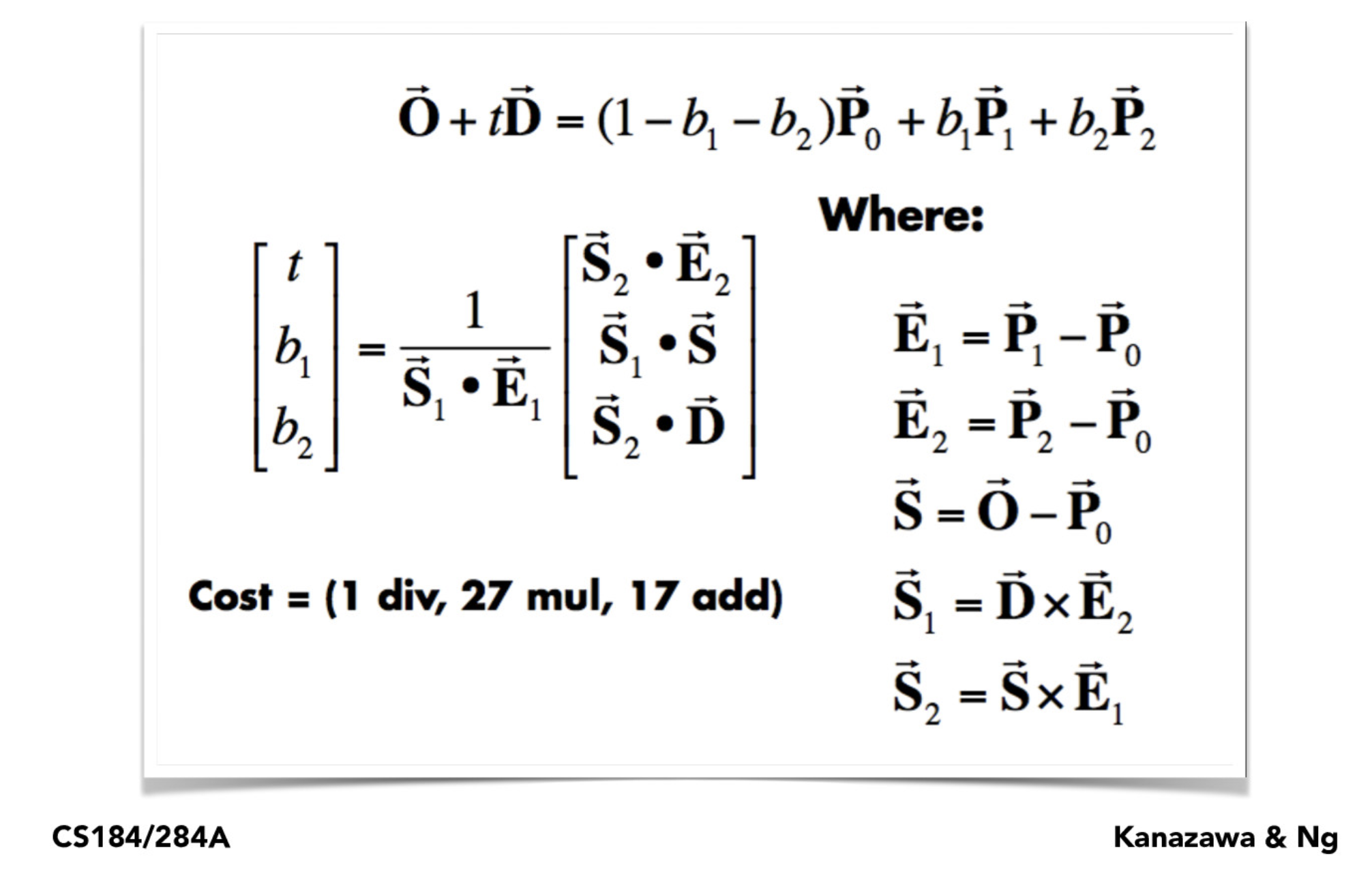
To optimize a bit the computation, we computed the barycentric coordinates only if the intersection time was valid. With the barycentric coordinates we can compute the average normal at the intersection point easily. The code is as follows:

  Vector3D E1 = p2 - p1;
  Vector3D E2 = p3 - p1;
  Vector3D S = r.o - p1;
  Vector3D S1 = cross(r.d, E2);
  Vector3D S2 = cross(S, E1);

  double divisor = dot(S1, E1);
  double t = dot(S2, E2) / divisor;

  if (t >= 0 && t >= r.min_t && t <= r.max_t) {  // intersects the plane with t in valid range
    double b2 = dot(S1, S) / divisor;  // baricentric coefficient for vertex 2
    double b3 = dot(S2, r.d) / divisor;  // baricentric coefficient for vertex 3
    double b1 = 1 - b2 - b3;

    if (b1 >= 0 && b2 >= 0 && b3 >= 0) {  // intersects the triangle!
      r.max_t = t;  // Update ray's max intersection time!
      isect->t = t;
      isect->n = b1 * n1 + b2 * n2 + b3 * n3;  // Let's get the mean normal at the intersection point
      isect->primitive = this;
      isect->bsdf = get_bsdf();
      return true;
    }
  }
  return false;

Results

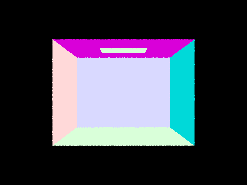
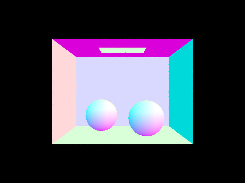
Here are a few .dae examples with normal shading:

CBempty.dae	CBgems.dae
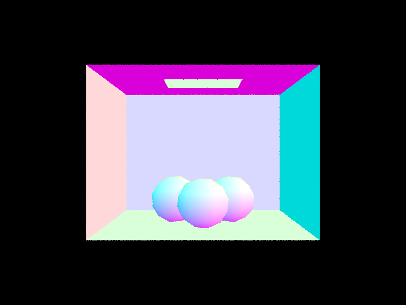CBspheres.dae

Part II: Bounding Volume Hierarchy (BVH)

BVH construction & heuristic

Iterating over each primitive in the scene is not scalable, therefore a better data structure was needed. We implemented a BVH structure with simple heuristics that allows us to reduce computation from an O(n) time complexity to O(log(n))!

To construct the BVH, which has a tree structure, we wrote the construct_bvh(std::vector<Primitive *>::iterator start, std::vector<Primitive *>::iterator end, size_t max_leaf_size) function, which starts with the root node and goes on recursively. On every recursive call, we first compute the node’s bounding box by combining the bounding box of each primitive in the subtree that starts from this node. To do this, we iterate the primitives in the subtree from start to end and used the Bbox::expand function. We also compute the mean centroid position for the elements in the bounding box, which will be used later in our heuristic. This part of the code looks as follows:

  BBox bbox;
  int num_elements = end - start;
  Vector3D mean_centroid = Vector3D();

  for (auto p = start; p != end; p++) {
    BBox bb = (*p)->get_bbox();
    bbox.expand(bb);
    mean_centroid += bb.centroid();  // might want to compute only if more than max_leaf_size elements
  }

  mean_centroid /= num_elements;
  BVHNode *node = new BVHNode(bbox);

If the number of elements (num_elements) under this node is less than the max_leaf_size, then we are in a leaf and we assign the node’s start and end iterators to the function’s input start and end. There’s nothing else to do here and we proceed to return the node:

  if (num_elements < max_leaf_size) {
    // if less than max_leaf_size elements just return with bounding box
    node->start = start;
    node->end = end;
    return node;
  }

Now, if we have more than max_leaf_size nodes, we need to choose along what axis to split our primitives and where within that axis to split. A simple heuristic we implemented consists of splitting the axis that has the largest length in the bounding box extent, and splitting at the centroid location of that axis. Finally, once we have the split, we assign the left and right child of the current node as the output of construct_bvh for each of the splits. This heuristic was both simple to implement and quick to run, and obtained good results. The code for this looks as follows:

  } else {  // more than `max_leaf_size` elements
   
    double max_extent = max(bbox.extent.x, max(bbox.extent.y, bbox.extent.z));
    double split_point;
    std::vector<Primitive *>::iterator bound;

    if (bbox.extent.x == max_extent) {  // split along X
      split_point = mean_centroid.x;
      bound = partition(start, end, [split_point](Primitive *primitive) {
                          return primitive->get_bbox().centroid().x <= split_point;
                        }
      );
    } else if (bbox.extent.y == max_extent) {  // split along Y
      split_point = mean_centroid.y;
      bound = partition(start, end, [split_point](Primitive *primitive) {
                          return primitive->get_bbox().centroid().y <= split_point;
                        }
      );
    } else {    // split along Z
      split_point = mean_centroid.z;
      bound = partition(start, end, [split_point](Primitive *primitive) {
                          return primitive->get_bbox().centroid().z <= split_point;
                        }
      );
    }

    if (bound - start == 0 || end - bound == 0){  // everyone has same centroid, just split in two here
      bound = start;
      for (int i = 0; i < (end-start) / 2; bound++, i++);
    }

    node->l = construct_bvh(start, bound, max_leaf_size);
    node->r = construct_bvh(bound, end, max_leaf_size);

  }

  return node;

In some rare cases, the centroid of all elements in the subtree was the same, which caused the initial version of this heuristic to fail. In this cases, we would just split the primitives in half. This happened just one case one level before the leaf level, where we had four elements left with the same centroid along the largest extent axis.

We also implemented another heuristic first, which would split just at the middle of the bounding box, but this heuristic tended to throw segfault more often. Finally, we also implemented a version that would split along the axis that would generate the most equal split. To do this, we would count how the split would distribute if separating along the subtree average primitive centroid.

Results

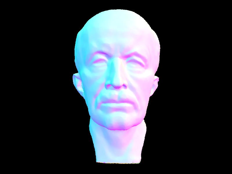
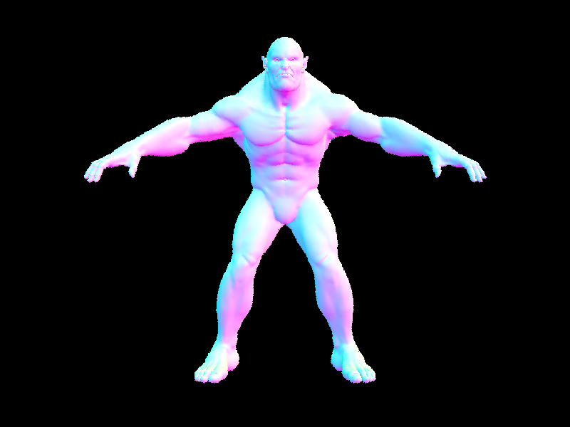
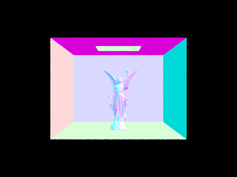
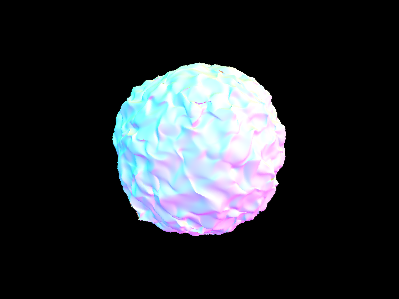
Here are some images with normal shading that are possible to compute super fast with our BVH acceleration.

maxplanck.dae	beast.dae
CBlucy.dae	blob.dae
wall-e.dae

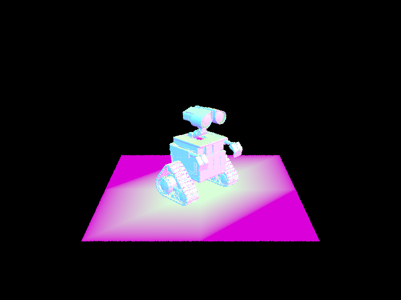BVH acceleration results and analysis

We benchmarked a few files in a 2019 MacBook Pro using 8 threads and producing an 800x600 image:

Filename	# of primitives	Render time without BVH	Render time with BVH
cow.dae	5856	20.12s	0.0457s
maxplanck.dae	50801	221.82s	0.0524s
beast.dae	64618	283.56s	0.0406s
CBlucy.dae	133796	Too long	0.0430s
blob.dae	196608	Too long	0.0558s
wall-e.dae	240326	Too long	0.0579s

As we can see, by using BVH acceleration we have that rendering time almost doesnt suffer when we increase the number of primitives. From the cow.dae to the maxplanck.dae we have about 10 times the number of primitives, and as a result the render without BVH takes about 10 times longer (which is what we expected! o(n)). On the other hand, the time with BVH implementation barely changes over all renderings. We would expect the time to increase around 25% from the cow to maxplanck (log(50801) / log(5856)), however, it seems that at this point the data structure is quite efficient that the bottleneck is in other operations in the pipeline. BVH is great!

Part III: Direct Illumination

Direct lighting function

We wrote two versions for direct lighting: Direct Lighting with Uniform Hemisphere Sampling and Direct Lighting by Importance Sampling Lights. In both approaches, we trace inverse rays: we cast a ray from the camera through a specific pixel until it intersects something in the scene. We then calculate how much light is reflected back towards the camera by calculating how much light arrived at that intersection point from elsewhere.

To estimate how much light at the intersection point, we use the following Monte Carlo estimator described in lecture:

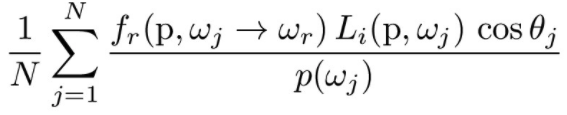
Here, p (hit_p in the code) is the intersection point, wr (w_out) is the outgoing direction, and w_j (w_in) is the incoming ray direction (which we will sample with two strategies).

Once we have an estimate of the incoming light we can use the reflection equation to calculate how much outgoing light will be.

Direct Lighting with Uniform Hemisphere Sampling

Here, we implemented estimate_direct_lighting_hemisphere. In this method, we estimate the direct lighting on a point by sampling wj uniformly in a hemisphere. Up to this task, we only check for direct illumination, so we want to check if the ray from hit_p in the sampled direction intersects a light source.

The code looks as follows:

    double ds = 1.0 / (double) num_samples;  // integrate over samples "ds"
    for (int i=0; i<num_samples; i++){
      Vector3D w_in = hemisphereSampler->get_sample();
      Ray ray = Ray(hit_p, o2w * w_in);
      ray.min_t = EPS_F;
      Intersection intersection;
      if (bvh->intersect(ray, &intersection)){
        L_out += isect.bsdf->f(w_out,w_in) * intersection.bsdf->get_emission() * cos_theta(w_in) * (2 * PI) * ds;
      }
    }

Direct Lighting by Importance Sampling Lights

Uniform sampling in the hemisphere produces noisy results since the approach is not efficient on the samples: we sample a lot of rays that don’t hit a light source and are wasted. However, as we increase the number of samples, we will inefficiently converge to the right noise-free solution.

Instead, we can do importance sampling! Here, we implement the estimate_direct_lighting_importance method, where we sample the lights directly rather than uniformly distributed directions. To do so, for each light in the scene, we sample directions between the light source and the intersection point hit_p. The code looks as follows:

    for (auto *light: scene->lights){
      samples_per_light = light->is_delta_light() ? 1 : (int) ns_area_light;  // if point light just sample once
      ds = 1.0 / double (samples_per_light);  // sample weight

      for (int i=0; i<=samples_per_light; i++){
        L_i = light->sample_L(hit_p, &w_in, &distToLight, &pdf);
        w_in_object = w2o * w_in;
        
        if (w_in_object.z >= 0){
          ray = Ray(hit_p, w_in);
          ray.min_t = EPS_F;
          ray.max_t = distToLight - EPS_F;
          if (!bvh->has_intersection(ray)){
            L_out += isect.bsdf->f(w_out, w_in_object) * L_i * cos_theta(w_in_object) * ds / pdf;
          }
        }
      }
    }

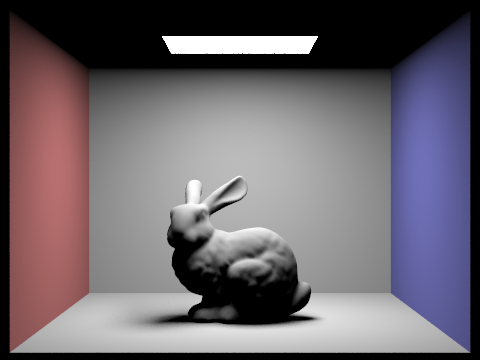
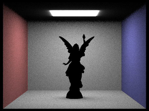
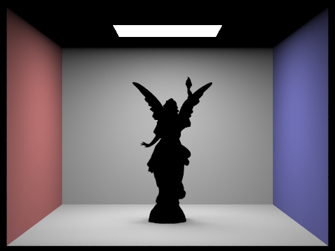
Results for both implementations fo direct lighting function

Here are some images rendered with both implementations of the direct lighting function. We can see that for CBlucy.dae we have not implemented the material and the for dragon.png hemisphere sampling completely fails since we have a point light source that is unlikely to get sampled.

Uniform Hemisphere Sampling	Importance Sampling Lights
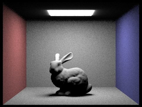
CBbunny.dae with -s 16 -l 8	CBbunny.dae with -s 16 -l 8
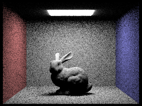CBbunny.dae with -s 64 -l 32	CBbunny.dae with -s 64 -l 32
CBlucy.dae with -s 64 -l 32 (Material not implemented!)	CBlucy.dae with -s 64 -l 32 (Material not implemented!)
dragon.dae with -s 64 -l 32 (Point light!)	dragon.dae with -s 64 -l 32

Effect of number of light rays with 1 sample per pixel

We compare the noise levels in soft shadows for multiple number of light rays (l) when using light sampling. The noise level reduces as we increase the number of light rays. This make sense as we are obtaining a better estimate of our integral which incorporates more directions as we increase the number of rays. This is particularly important for the soft shadows, as only rays from some directions will actually make it to the source light.

l=1	l=4
l=16	l=64

Analysis

We can clearly see a big improvement by using importance lighting sampling instead of hemisphere sampling. Importance sampling allows us to focus our samples on rays that will actually contribute to the integral estimate, allowing us to reduce noise and avoid complete fails where sampling the light source is unlikely (e.g. point source light as in dragon.dae).

Part IV: Global Illumination

Implementation of the indirect light function

In this part, we implemented the algorithm to perform indirect light rendering. Recall from Part 3, where we successfully implemented one_bounce_radiance function. Here, we recursively call that function to estimate the higher bounces. Specifically, assume we have the intersection for the first bounce, we can create a new ray starting from the intersection with a sampled input light direction. Then, we can recursively call the one_bounce_radiance on top of the new rays. To save the computation, we also implemented Russian Roulette for unbiased random termination.

Our codes:

Vector3D PathTracer::at_least_one_bounce_radiance(const Ray &r,
                                                  const Intersection &isect) {
  Matrix3x3 o2w;
  make_coord_space(o2w, isect.n);
  Matrix3x3 w2o = o2w.T();

  Vector3D hit_p = r.o + r.d * isect.t;
  Vector3D w_out = w2o * (-r.d);

  Vector3D L_out = one_bounce_radiance(r,isect);

  double termination = 0.4;

  if (r.depth == 1)
  {
      return L_out;
  }

  Vector3D wi;
  double pdf;

  Vector3D f = isect.bsdf->sample_f(w_out,&wi,&pdf);
  Vector3D wi_world = o2w * wi;
  Ray next_ray = Ray(hit_p,wi_world);
  next_ray.depth = r.depth - 1;
  next_ray.min_t = EPS_F;
  Intersection next_intersection;
  bool next_isec_bool = bvh->intersect(next_ray,&next_intersection);
  if (next_isec_bool)
  {
      if (r.depth == max_ray_depth)
      {
          L_out += at_least_one_bounce_radiance(next_ray,next_intersection)*f* cos_theta(wi)/pdf;
      }
      else if (coin_flip(1-termination))
      {
          L_out += at_least_one_bounce_radiance(next_ray,next_intersection)*f* cos_theta(wi)/(pdf*(1-termination));

      }
  }
  return L_out;

Results

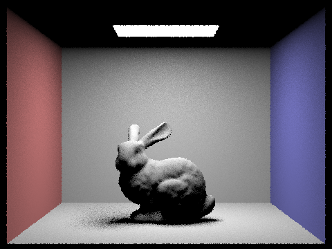
1. Images rendered with global (direct and indirect) illumination (Using 1024 samples)

Direct illumination (m=1)	Indirect illumination (m=5)
Bunny Results	Bunny Results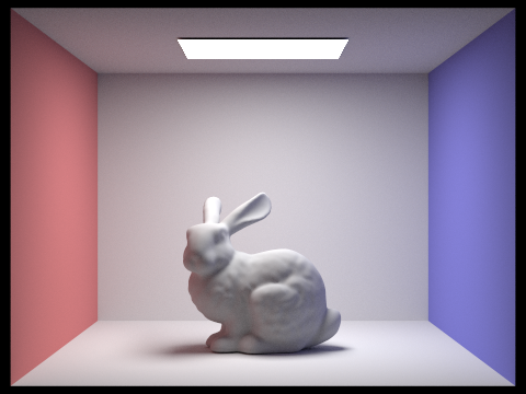
Sphere Results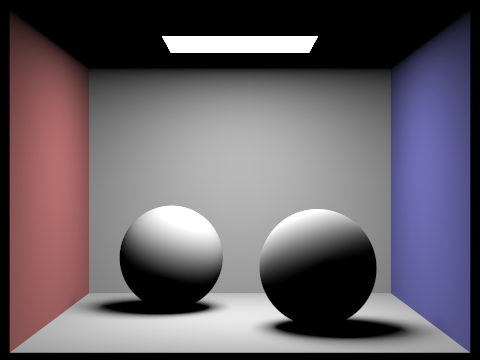	Bunny Results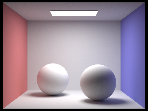

2. Images rendered with only direct illumination and only indirect illumination (Using 1024 samples)

Only Direct illumination (m=1)	Only Indirect illumination (m=3)
Bunny Results	Bunny Results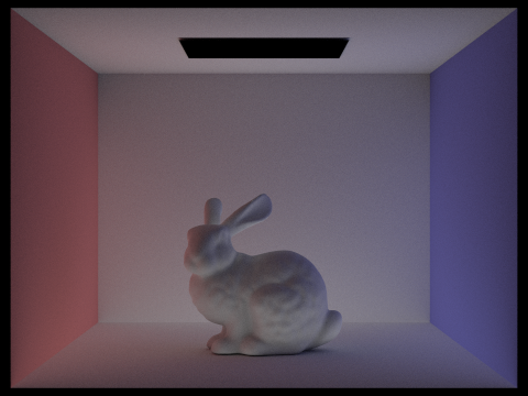

3. Images rendered with different max_ray_depth (Using 1024 samples)

m=0	m=1
Bunny Results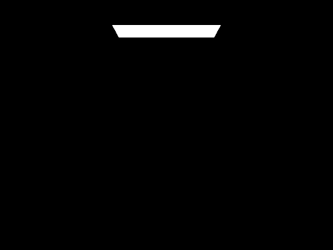	Bunny Results
m=2	m=3
Bunny Results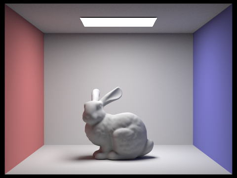	Bunny Results
m=100
Bunny Results

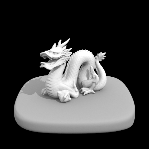
4. Images rendered with different sample-per-pixel rates. (m=3)

s=1	s=2
Dragon Results	Dragon Results
s=4	s=8
Dragon Results	Dragon Results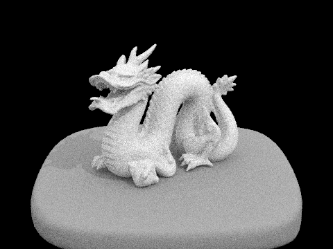
s=16	s=64
Dragon Results	Dragon Results
s=1024
Dragon Results

Part V: Adaptive Sampling

To implement the adaptive sampling, we computed the average mu and variance sigma^2 every samplesPerBatch samples, and terminate the sampling when I<=maxTolerance*mu, where I = 1.96* sqrt(sigma_2)/sqrt(actual_sample). Our implementatin codes:

void PathTracer::raytrace_pixel(size_t x, size_t y) {
  int num_samples = ns_aa;          // total samples to evaluate
  Vector2D origin = Vector2D(x, y); // bottom left corner of the pixel
  Vector3D illum_average = Vector3D();
  double weight = 1/(float)num_samples;
  double s1 = 0;
  double s2 = 0;
  int actual_sample = 0;
  for (int i = 0; i< num_samples; i++)
  {
      if (i!=0 && (i % samplesPerBatch) ==0)
      {
          double mu = s1/double(actual_sample);
          double sigma_2 = (1/(double(actual_sample)-1))*((s2)-(s1*s1/(actual_sample)));
          double I = 1.96* sqrt(sigma_2)/sqrt(actual_sample);
          if (I<=maxTolerance*mu)
          {
              break;
          }
      }
      Vector2D xy_sub = gridSampler->get_sample();
      double x_image = (x+xy_sub.x)/sampleBuffer.w;
      double y_image = (y+xy_sub.y)/sampleBuffer.h;
      Ray ray_sample = camera->generate_ray(x_image,y_image);
      ray_sample.depth = max_ray_depth;
      Vector3D radiance = est_radiance_global_illumination(ray_sample);
      s1 += radiance.illum();
      s2 += (radiance.illum())*(radiance.illum());
      illum_average = illum_average + radiance;
      actual_sample++;

  }
  illum_average = illum_average/actual_sample;


  sampleBuffer.update_pixel(illum_average, x, y);
  sampleCountBuffer[x + y * sampleBuffer.w] = actual_sample;


}

Results

Images rendered with adaptive sampling.

Rendered image	Sampling rate
Bunny Results	Bunny Results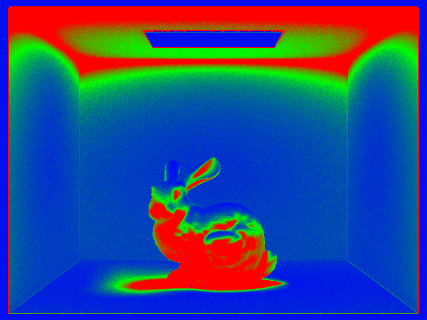

We can see clearly visible differences in sampling rate over various regions and pixels.

Note on collaboration

We’ve been working together since the first project, as well as collaborating in research in our lab. For the CS284A course projects we’ve worked independently on the each task of the coding part of the assignment (in separate branches), and we would discuss issues / point out bugs / discuss alternative implementations. At the end we would either merge one of the two branches into master or combine parts of each branch. Now, for the write-up, we usually split the tasks. This has been working since we both have tight schedules and allows both of us to dig into the code (and learn in this process), but we think it might be worth trying to more actively collaborate to speed up the process.