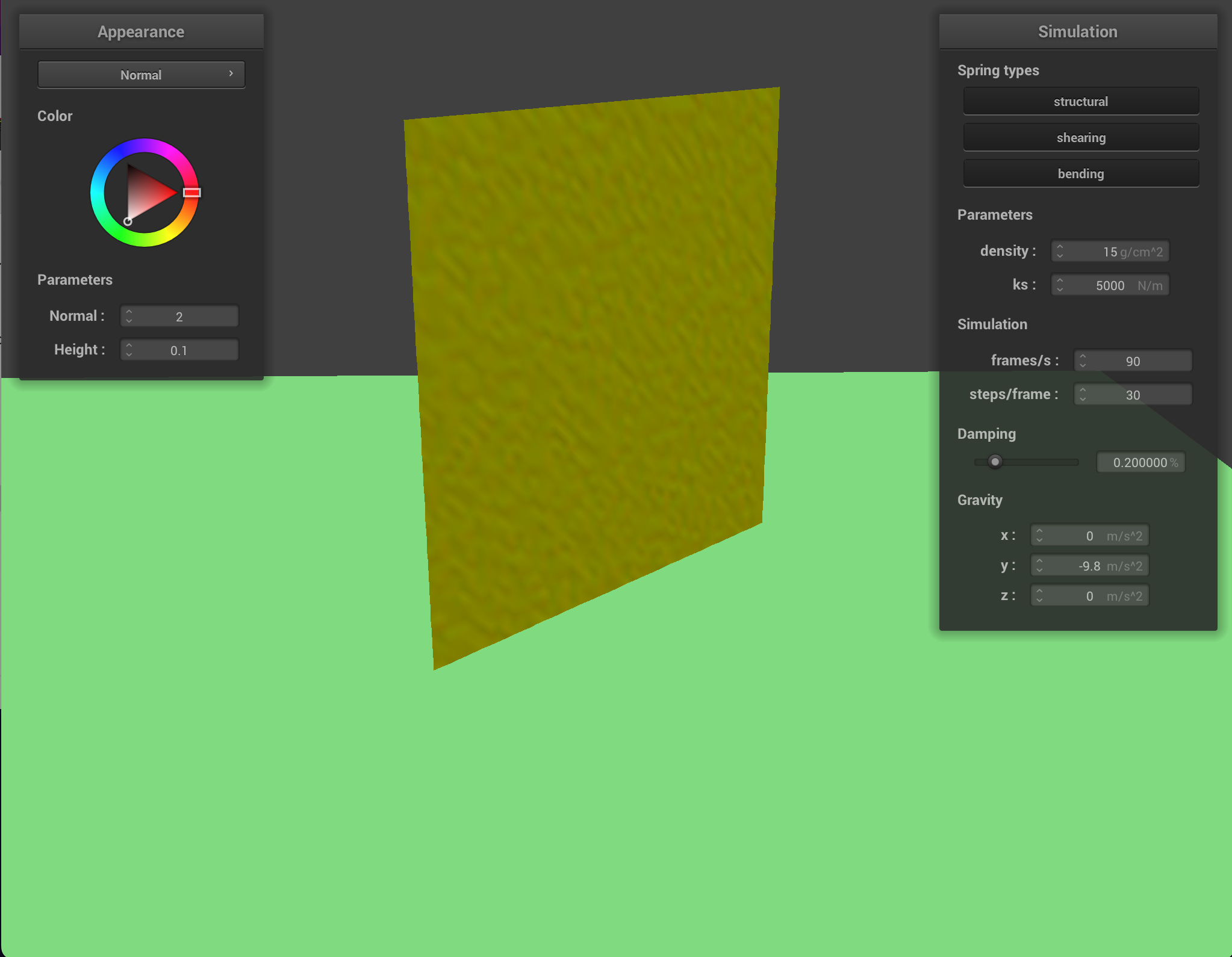
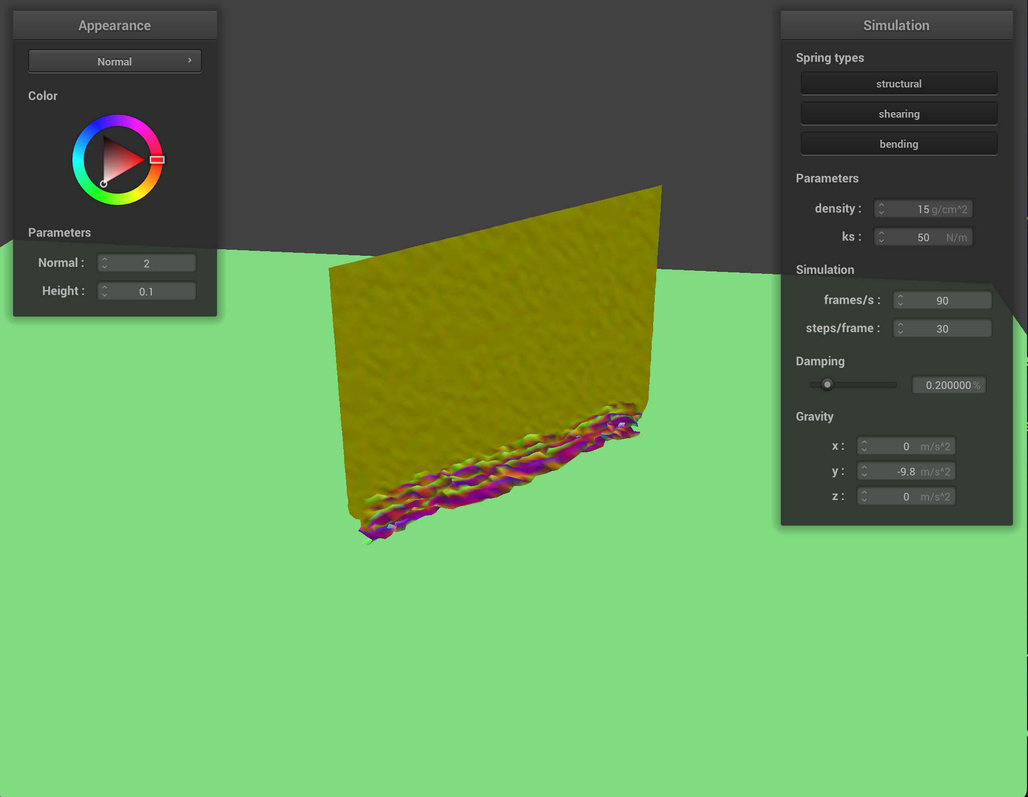
The spring constant in Hooke's Law is an indicator of the stiffness of the spring. If we decrease the spring value from ks = 5000 to ks = 100. As shown in the image below, the cloth has more wrinkles but smaller and the texture seems more smooth and less stiff. If we increase the spring constant to ks = 50000, the overal spring movement is stiff and there are less wavey wrinkles on the cloth.

Another variable in our simulation is density. If we decrease the density from 15 to 1. With density being small and surface are stay the same, the cloth becomes lighter, which is shown in the image below. By contrast, if we increasr the density to 100, the cloth is heavier. We can observe from the image that the pinned side of the cloth is pushing down the cloth significantly and exerting pressure due to its weight.

The last variable that impact the simulation is the damping constant. Damping variable influences the time it takes for the Cloth to stop oscillating. If we set the damping value to be 0, the cloth will keep oscillating and the energy does not dissipate. As we increase the value of damping, the cloth will come to a stop more and more quickly because the energy loss increase with the damping value. When we set damping value to 1, the oscillation immediate stops and the cloth comes to a stop.

The images below are pinned4.json where the four endpoint of the cloth is pinned.

Part III: Handling collisions with other objects

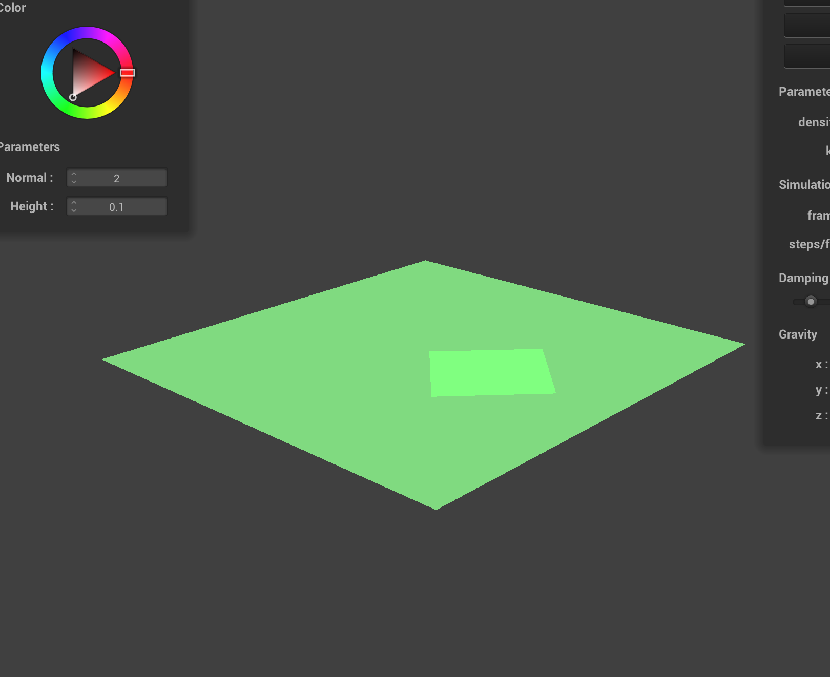
In part 3 of the project, we implemented the collision of sphere and plane. For both collision method, we calculate the tangent_point which is the point of intersection and update the current position by applying correction_vector on the last position.

The image below is a series of cloth falling onto a sphere with different spring constants. By observation, we can see that with smaller spring constant, the cloth is more tight around the sphere and the rendering gives out a sense that the cloth is heavy and pushing down on the sphere. On the other hand, with a larger spring constantm, the cloth is more flexible and dangling around the sphere. It gives a feeling that the cloth is relatively light in weight.

Below is the rendering of the plane.json where the cloth falls onto a plane and collide. The implementation of plane collider is similar to the sphere collider except for the surface offset which we use to account for the slight displacement of point mass crossing over the plane.

Part IV: Handling self-collisions

In this part of the project, we deal with the self collision between the point mass in the cloth to achieve more realistic simulation. The first two functions we have implemented is hash_position() and build_spatial_map(). For hash_function, I use pow(31,2)* x + pow(31,1) * y + pow(31,0) * z as the hash function since 31 is a prime so it will create less collision. After that,we fill in the build_spatial_map(). We iterate through all point mass and calculate the hash value of the point mass and fill it in a hash table. The purpose of this is to detect the point mass that are really close to each other and will be used to computation of self-collision later. For the last function, we implement self_collide(). For the specific point mass, we look up the hash table with its hash value to get the candidate that the point mass will collide. Then we determine whether it is 2 * thickness apart from each other. If it is less than 2 * thickness, we will apply correction so that they are apart from each other 2 * thickness away.

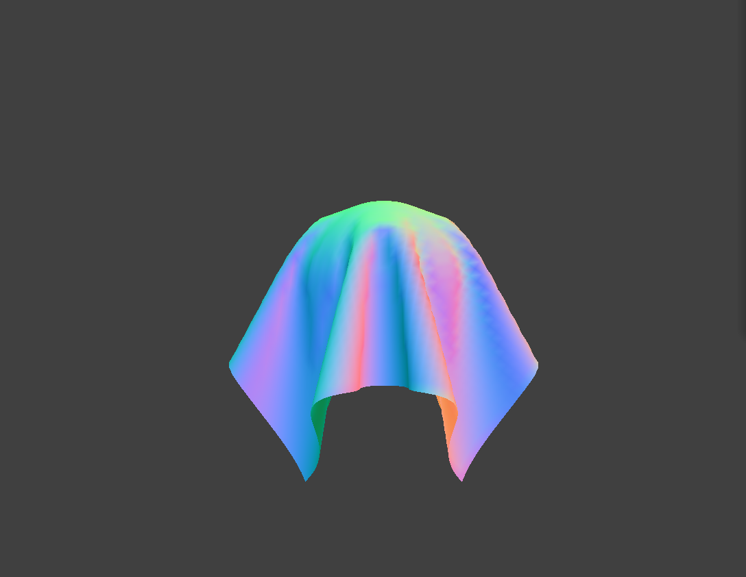
Beginning the simulation, the cloth starts to collide with each other, creating the wave shapes on the cloth. When it falls on the the ground different layers of cloth emerges as a result of collisiion and due to the spring constant, the cloth will do some foldings until it comes to rest.

Below is a series of image with spring constant ks = 50, 5000, and 50000. We can observe that as the spring constant increases, the cloth becomes more smooth and less wavey, which means that the spring does not bounce that often. For ks = 50, we see that the cloth is constantly folding and bounce a lot of time when it falls down.

Below is a series of image with density ranging from 1, 15, to 50. We can see that with low density, there is not much force pressing down the cloth and the cloth looks like a paper falling down. When the density is really high, we can see that the cloth is pressed down to the ground quickly when it touches the floor. It also folds itself more often.

Part V: Shaders

In the last part of the project, we implement a variety of shaders. Shader program is a program that utilizes the computing power of GPU and will run in parallel. The shader programs takes in color or texture map and will output information such as color or transformation on vertex and pixel. There are two types of shaders: vertex shader and fragment shader. Vertex shader generally apply transformation to the vertices after rasterization. Fragment shaders uses the geometric attributes computed from the vertex shaders and use it to color the rendering. In order to generate lighting and material effect, we first use the vertex shaders to transform the vertices. Then we will apply the fragment shader to piece together the fragment and fill in the color.

For Blinn-Phong shading, we stack up three types of shadings: Specular, Diffuse, and Ambient. Specular shading is mostly the reflection of the surface, its intensity depends on the viewing direction. Diffuse shading depends on the view direction and the Ambient shading does not depend on anything. It adds color to the overall illumination. By adding the three shadings up, we get Blinn-Phong shading.

For texture mapping, we simply use texture(sampler2D tex, vec2 uv) to apply the texture at given u-v coordinate, I downloaded the texture of wood from Internet and apply it to the cloth rendering.

Below is a comparison between Bump Mapping and Displacement Mapping. For both mapping, we calcualte the tangent-bitangent-normal (TBN) matrix and apply it to the local space normal to get our normal and pass it as a variable for Blinn-Phong shading.

We can see that with low value of height, both bump mapping and displacement mapping looks similar. However, if we increase the height, the wrinkles of the cloth with displacement mapping becomes unrealistic since the vertices of the cloth are transformed. In my opinion, the bump mapping seems more realistic.

With low coarseness, the difference between the bump and the displacement is little. There are some sharp bumps within the displacement mapping. At high coarseness,the bump map is a better shading program as the displacement shading creates more sharp edges which results in inaccuracy.

The last shading we do is Environment-mapped Reflections. We implement by using the formula of reflection from the last project and calcuate w_in and w_out and applies to texture map accordingly.