Overview
In this project, we implemented a simulation of cloth which includes a spring and mass system. In order to do that, we constructed a mass and spring system, explored how cloth collides with the ground or different objects in vertical and horizontal orientations. We also included various shading mechanisms such as Diffuse, Blinn-Phong, Texture Mapping, Bump and Displacement Map, and Mirror Shaders.
Part 1: Masses and Springs
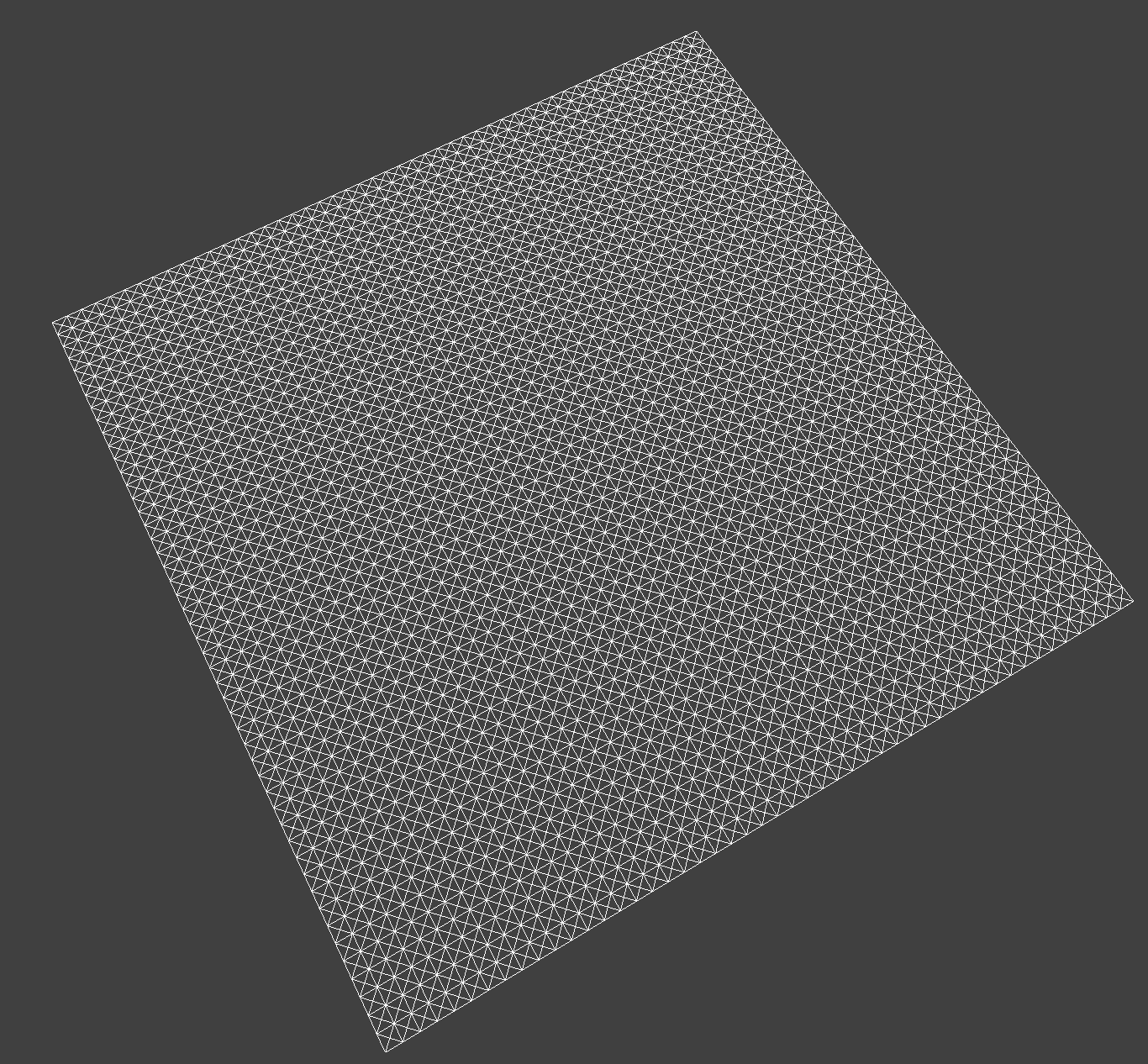
In our implementation for part 1, our goal was to divide a cloth of desired dimensions and parameters into point masses connected by springs. We first created an evenly spaced grid of masses that spanned width and height lengths. We separated out our code into horizontal and vertical orientation. If the cloth was horizontal, we set the y coordinate of point masses to 1; if the cloth was vertical, we generated a small offset to use for the z coordinate. We also maintained a Boolean called pinned which keeps track of whether or not we’ve included the point mass’s index to the cloth’s pinned vector. Once all the point masses are stored in the point_masses vector, we applied structural, shear, and bending constraints using springs. The structural, shearing, and bending constraints exist differently depending on the location of the point mass and its adjacent point masses.
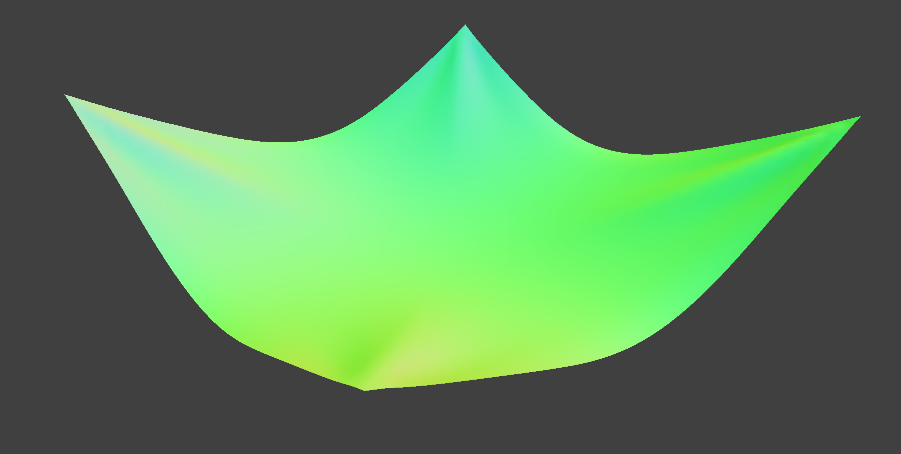
Here's an image of the cloth wireframe:
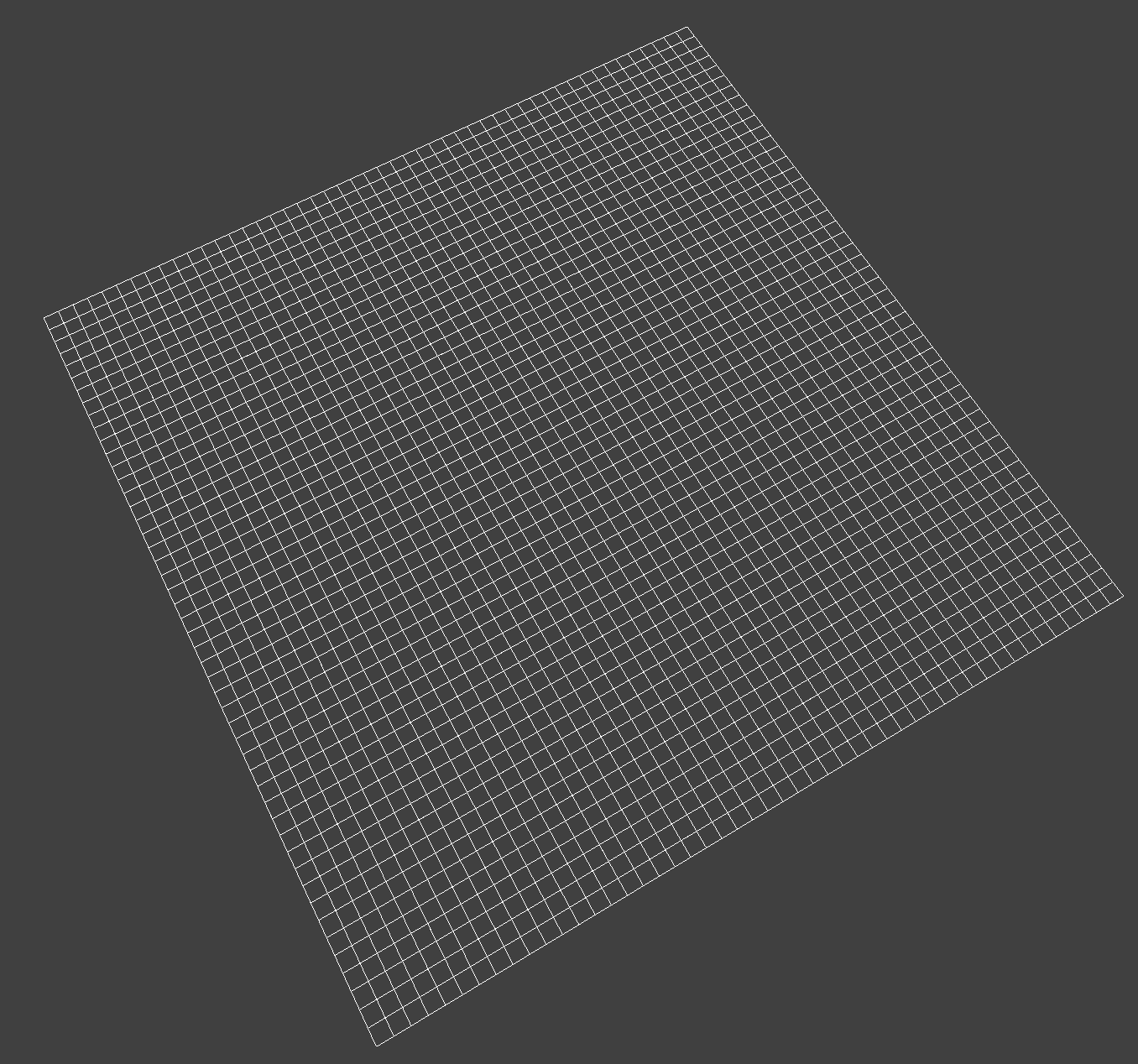
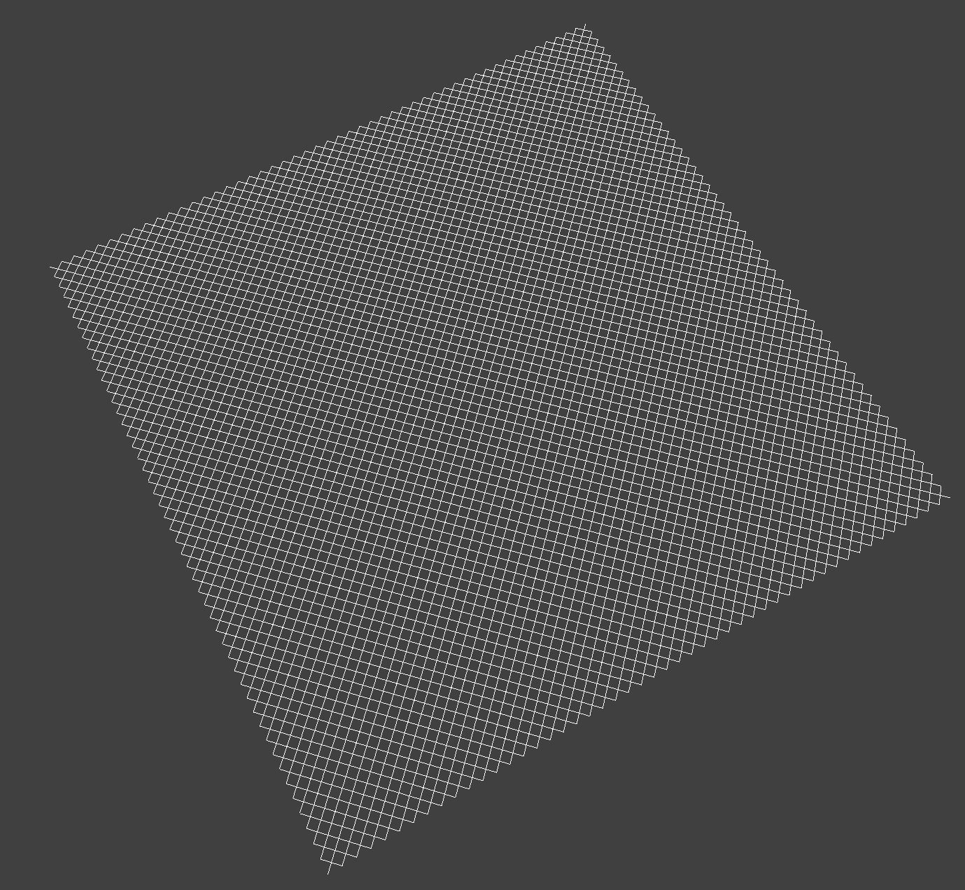
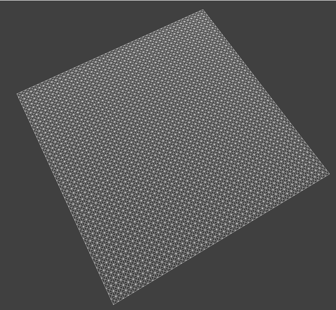
Below are images of spheres rendered with and without shearing constraints:
|
|
| |
|
Part 2: Simulation via Numerical Integration
For part 2, our goal was to simulate the cloth using numerical integration. This means that we needed to look at the physical equations of motion which could then be applied to the cloth’s point masses. By the end of this, we would know how the cloth moves at each time step.
First, we compute the total force that acts on each point mass. In order to do that, we use the external_accelerations and mass to calculate the total external force, which is applied to every point mass. Next, we want to compute the spring correction forces which can be found using Hooke’s Law. We iterate through each spring and if the spring’s constraint type is disabled, we simply skip it; we check this using enable_structural_constraints. We also need to make sure that we apply the force Fs to a point mass and the opposite force to the other point mass so that there are equal and opposite forces.
We then compute the new mass positions using Verlet’s Integration. We use the given equation which includes damping to simulate loss of energy. If the point pass is pinned, we don’t do anything; otherwise, we update the value of the mass position according to Verlet’s Integration.
In the final part of this section, we added a constraint feature to the simulation. We essentially correct the 2 point masses such that the length of the spring is no more than 10% greater than its rest_length. For each point mass, we only apply half the correction so that they sum to be 1 correction. If one point mass is pinned, we apply the correction just to the other point mass. If both are pinned, we do not apply the correction at all.
Effect of Ks: Changing the spring constant ks will impact how flexible or stiff the cloth is. A smaller ks correlates to a more flexible cloth whereas increasing ks causes the cloth to be more stiff. When we have a very low ks, the cloth was very flexible and somewhat wrinkly at the beginning and then towards the end, bounced around a bit. This is due to the springs being stretchier. With a high ks, the cloth was not wrinkly at the beginning and when it falls, it seems to just have one bending portion at the end. Compared to the default parameters, the cloth with a higher ks did not show many wrinkles.
Effect of Density: When we test different densities, we can see that a density of 1 makes the cloth feel very light as compared to increasing the density to 1000, which makes the cloth feel heavy. A higher density cloth moved around a lot more after falling whereas the smaller density cloth stayed in place more. From the beginning to the end, the smaller density cloth was faster and more flowy; the higher density cloth was still moving at the end and almost had a ripple effect. Compared to the default parameters, the cloth with a higher density just falls slower.
Effect of Damping: For damping, a smaller value meant that we were losing less energy and a higher value meant that we were losing more energy. With a damping value of 0, the cloth fell much faster and wavered back and forth towards the end with more energy. A damping value of 1 caused the cloth to fall a lot slower and not waver back and forth. Instead, it mainly stayed in place at the end. Compared to the default parameters, the cloth with a damping value of 0 had the cloth significantly moving back and forth to the point where it was no longer fully visible in some areas.
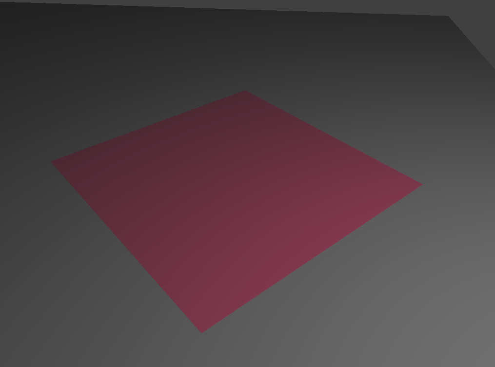
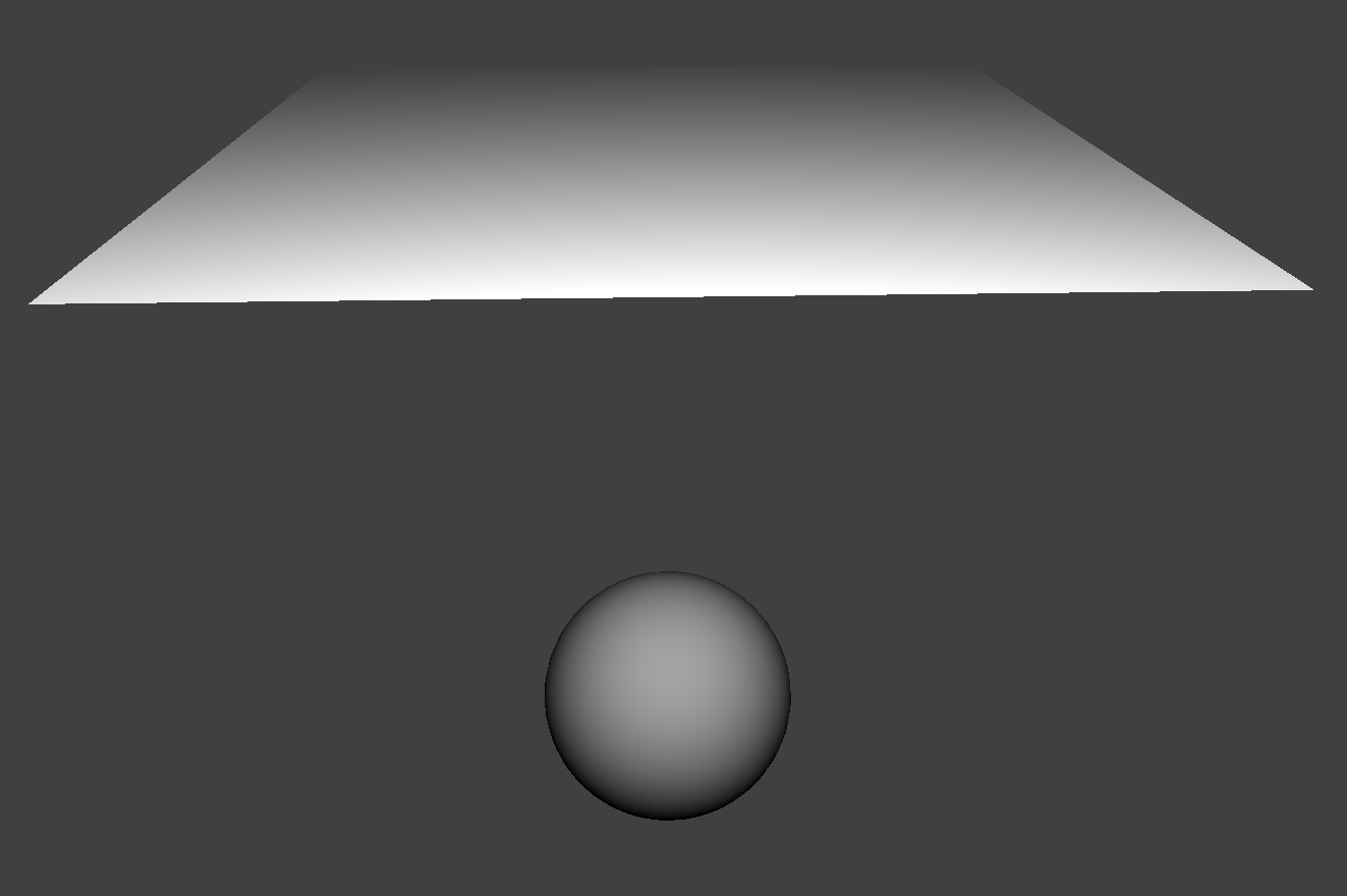
Part 3: Handling Collisions with other Objects
Now, we will be adding support collisions for the cloth with other objects such as spheres and planes. To handle collisions with spheres, we essentially take a point mass and adjust its position if it’s within the sphere. If the point mass intersects with or is inside the sphere, we bump it to the surface of the sphere by first computing where the point mass would’ve intersected and extending its path. We also compute the tangent point so that we can extend its path between the sphere’s origin and point of intersection. Next, we compute the correction vector which will be applied to the point mass’s last_position; this is what helps the vector reach the tangent point. Lastly, we set the position to last_position and we account for variables such as friction. Next, we worked on handling collisions with planes. The overall concept to handling collisions with spheres is extremely similar to planes. We just use a different method to figure out whether or not the cloth has intersected the plane. We know that if a mass has crossed over the plane in thie last step or if pm.last_position is not on the same side as pm.position, there is an intersection and we must apply the correction vector. This is what will bump the cloth onto the right side of the plane.
|
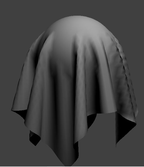
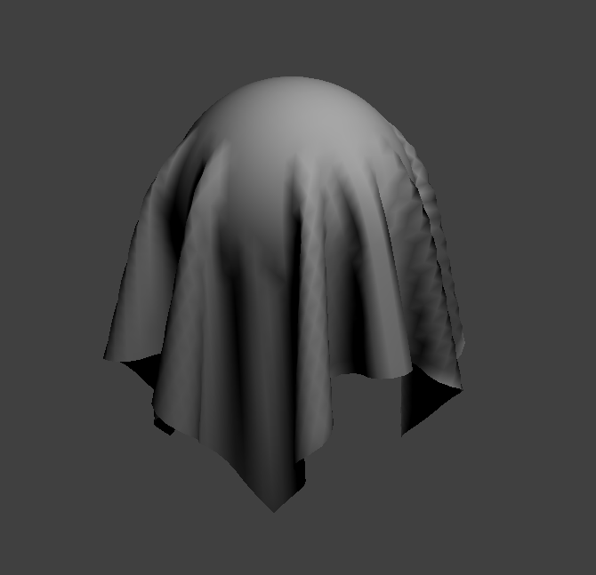
Here are images of the shaded cloth in its final resting state with Ks = 500, 5000, and 50000.
For ks = 500, the cloth is a lot “looser” which is why it is draped so closely to the sphere. On the other hand, the image with ks=50000 appears to have a much stiffer cloth due to the increased stiffness of the springs. This is why the cloth is not as closely draped to the sphere; the stiffness of the cloth prevents it from smoothly draping onto the sphere.
|
|
|
Part 4: Handling Self-Collisions
In part 4, we handle self-collisions of the cloth simulation. Without handling self-collisions, the cloth may clip through rather than falling normally. To implement self-collisions, we use spatial hashing techniques. First, we worked on hash_position which is a function that takes a point mass’s position and maps it to a float. The float uniquely represents a 3D box volume. To do this, we partitioned the space with the dimensions w, h, and t. We calculated w, h, and t as follows: w = 3 * width * num_width_points, h = 3 * height * num_height_points, t = max(w, h). We also made sure to check whether or not the cloth was horizontal or vertical; if the cloth was vertical, we swapped the h and t values. Using these values, we truncated the position coordinates to the closest values of the 3D box. We finally returned the sum of these values in a way such that we can use a unique key in our hash table.
The next step is to build a spatial map. This process is relatively straightforward but we essentially recurse through the point masses and use the hash_position method to populate our map.
Lastly, we implemented self_collide which uses the hash map we populated to search up potential collisions of a point mass. For each pair of point masses and potential collision point masses, we check to see if they are within 2*thickness distance apart. If they are, we compute a correction vector which makes it so that the pairs are 2*thickness distance apart. Otherwise, we just move on to the next pair. We also scale down the final correction vector by simulation_steps which improves the accuracy.
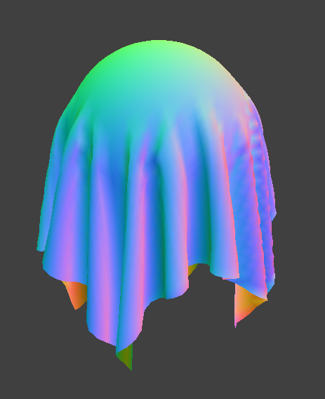
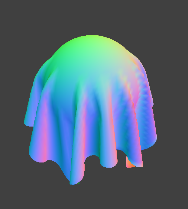
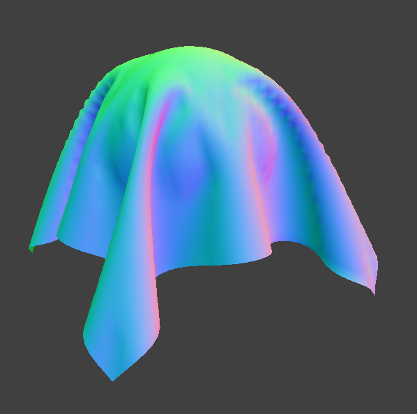
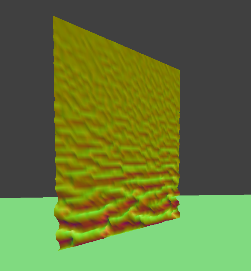
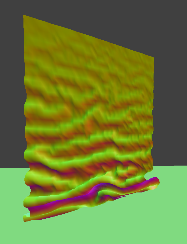
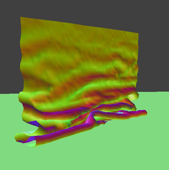
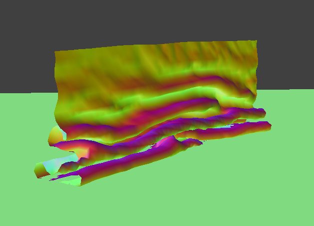
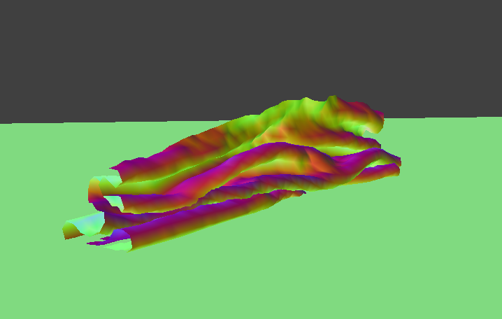
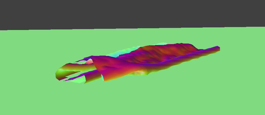
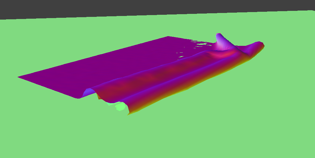
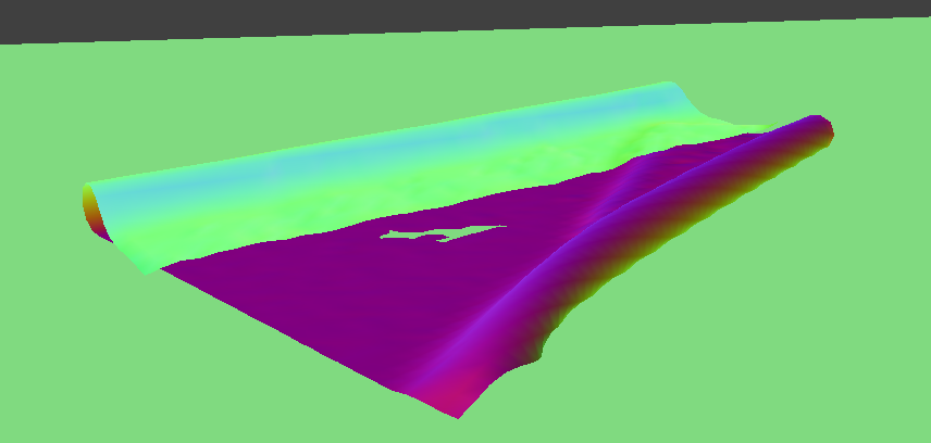
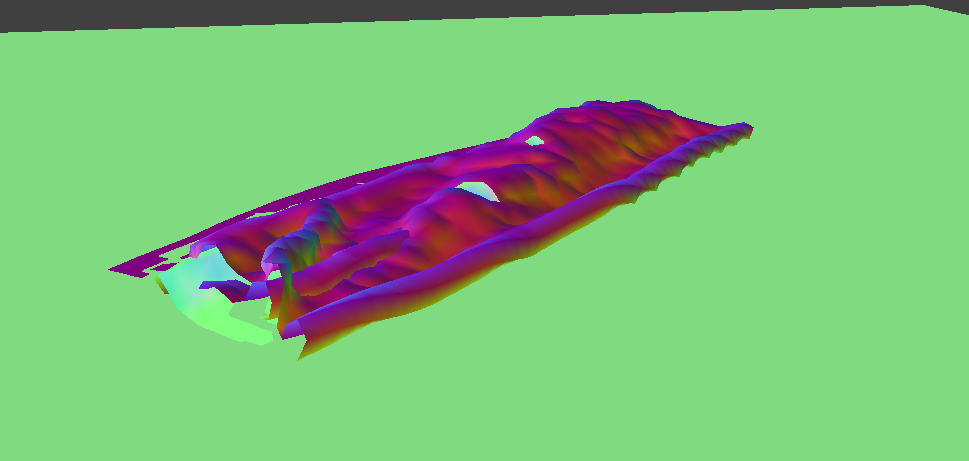
Here are images of how the cloth falls on itself from the early stage to a restful state:
|
|
|
|
|
|
Varying ks effect on behavior of cloth as it falls on itself: Increasing ks causes the cloth to be a lot stiffer and not bounce around as much as the cloth falls on itself. It also arrives at a resting position much sooner than a smaller ks and does not unfold. A lower ks causes the cloth to be a lot bouncier due to the springs. As the cloth falls, it has many more folds than a larger ks. It also bounces around more before reaching a resting position.
|
|
Varying Density effect on behavior of cloth as it falls on itself: Increasing the density causes the cloth to be more silky and it also falls in smaller folds. A lower density causes the cloth to fall in larger folds.
|
|
Part 5: Shaders
In our implementation for diffuse shading, our goal was to see what diffuse objects would look like under light. We used the formula Ld = kd(I/r^2)*max(0, n dot l) to calculate diffuse light.
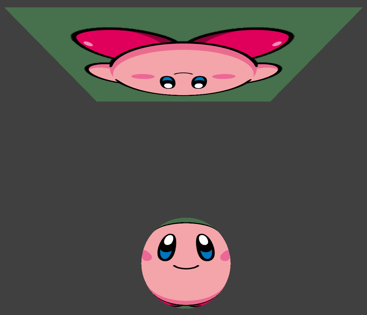
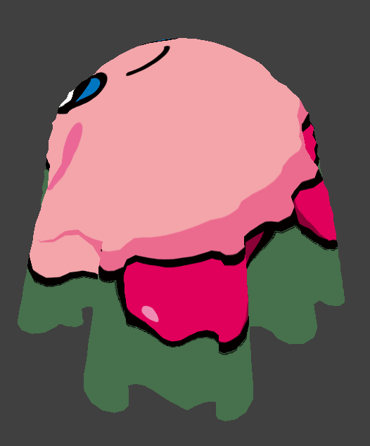
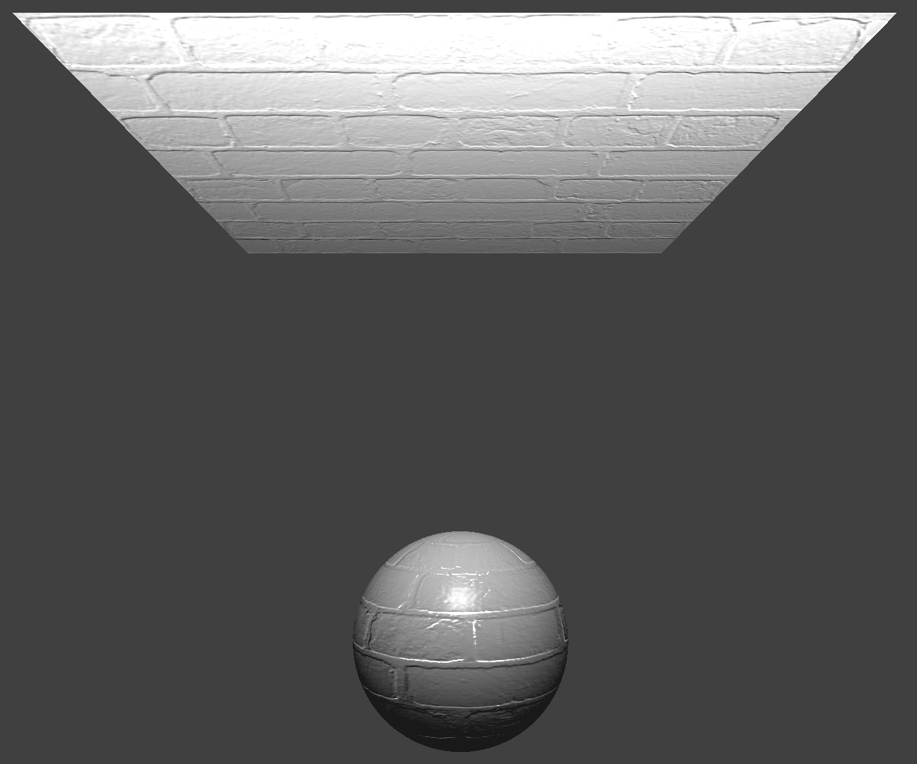
Next, we implemented texture mapping which is when we sample from the u_texture_1 uniform using the built-in texture function. Essentially, the texture function samples from the texture space coordinates.
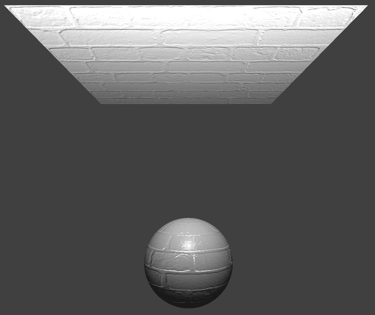
In this next section, we created bump and displacement maps. For bump mapping, our goal was to simulate bumps on an object by modifying the normal vectors. We modified the fragment shader in order to shade the surface for bump mapping. For displacement mapping, we modify the vertex shader in addition to the fragment shader. By modifying the vertex shader, we are also displacing the vertices instead of just the surface.
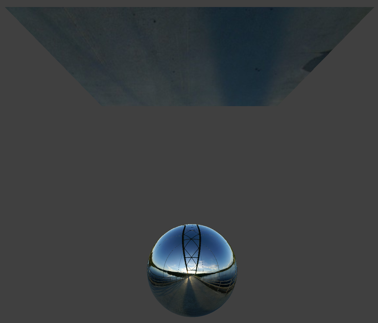
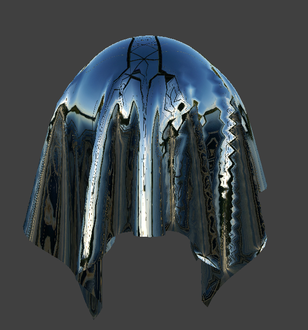
Lastly, we created environment-mapped reflections which provide a mirror-like effect. We used an environment map to approximate the incoming radiance sample. Since we know the camera’s position and fragment’s position, we can compute the outgoing ray which we then reflect across the surface normal. We then sampled the environment map to get the incoming direction wi.
A shader is a program that is isolated from the actual program, but it runs simultaneously with the GPU. Essentially, it takes an input and returns a single 4D vector. Vertex shaders work by transforming the positions of shapes into 3D drawing coordinates. On the other hand, fragment shaders compute the rendering of a shape’s colors. They both work together to provide information regarding position and color which gives the lighting and material effects.
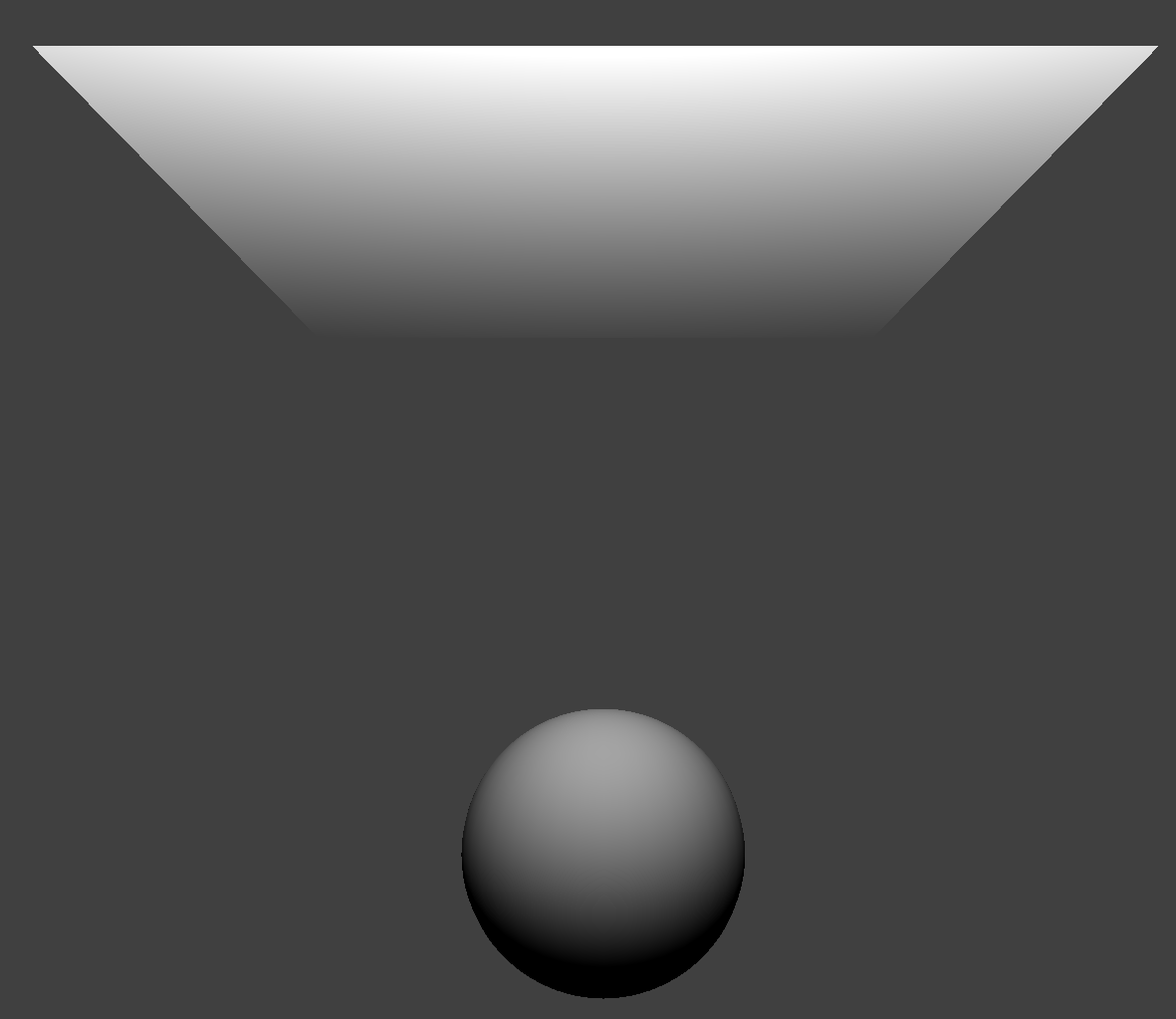
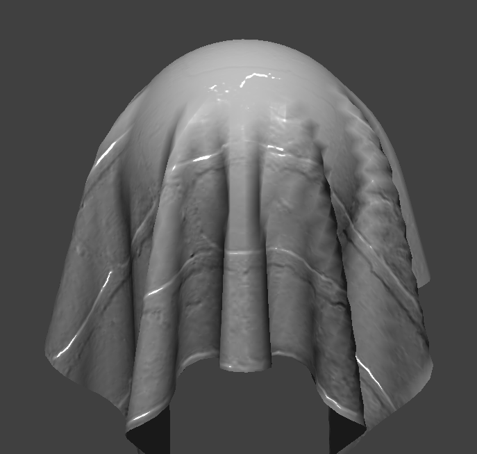
The Blinn-Phong Shading Model combines ambient, diffuse, and specular reflection. We implemented it by summing together each of these values. The equation we used is L = kaIa + kd(I/r^2)*max(0, n dot l) + ks(I/r^2)max(0, n dot h)^p.
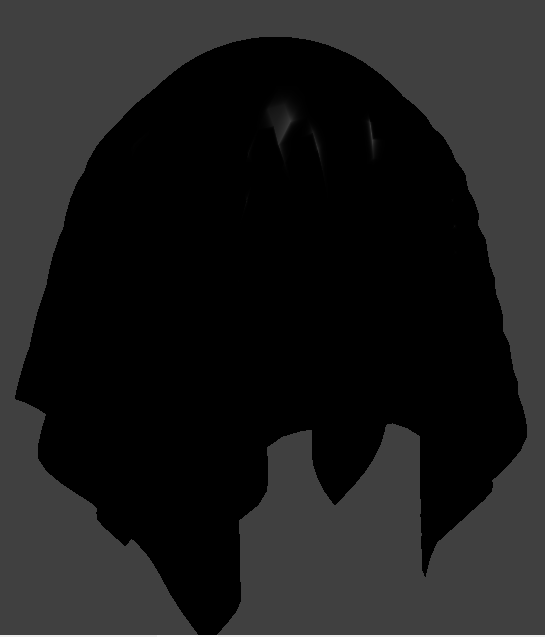
Here are images with the Blinn-Phong Shader:

|
|
|
|
|
|
|
|
Here are images of the Texture Mapping Shader:
|
|
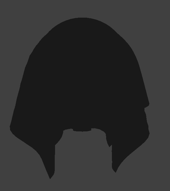
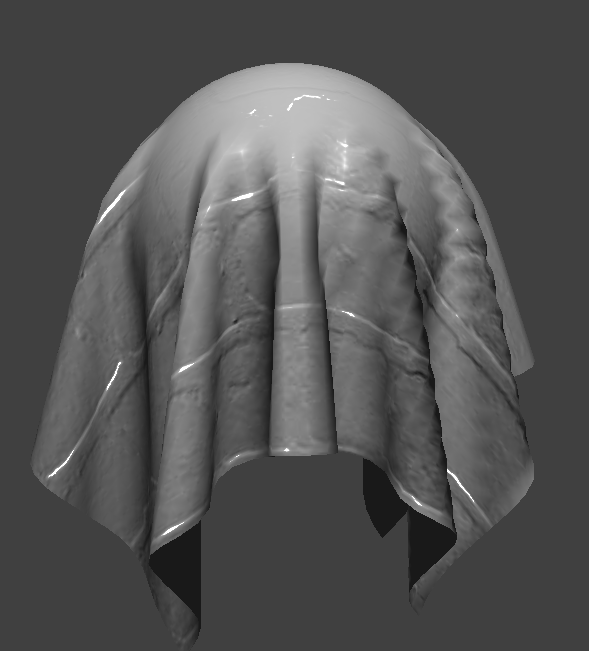
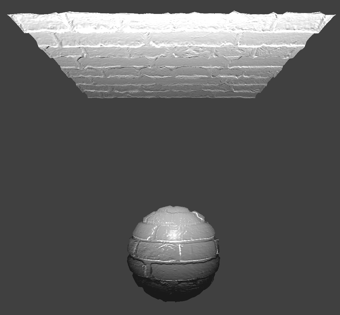
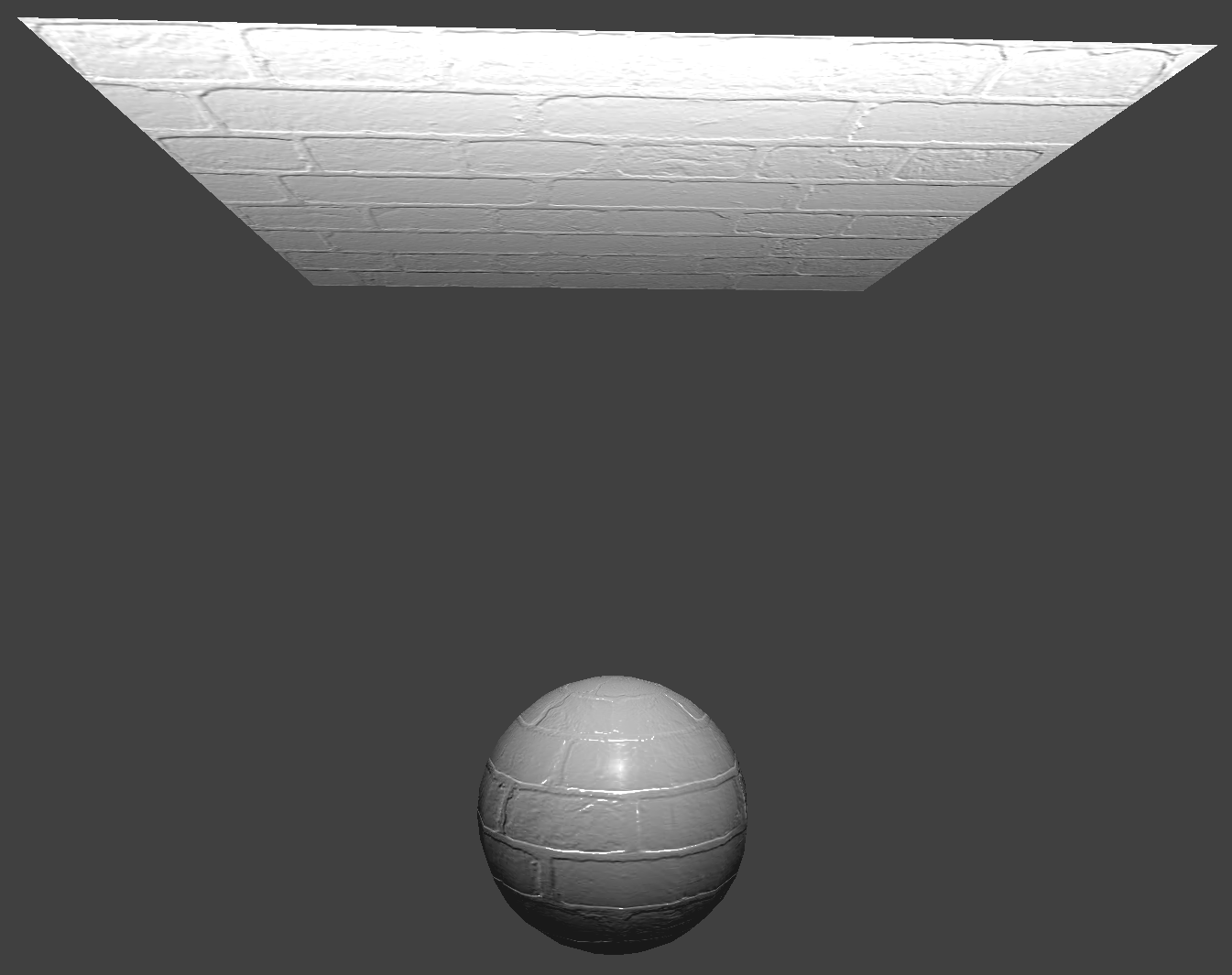
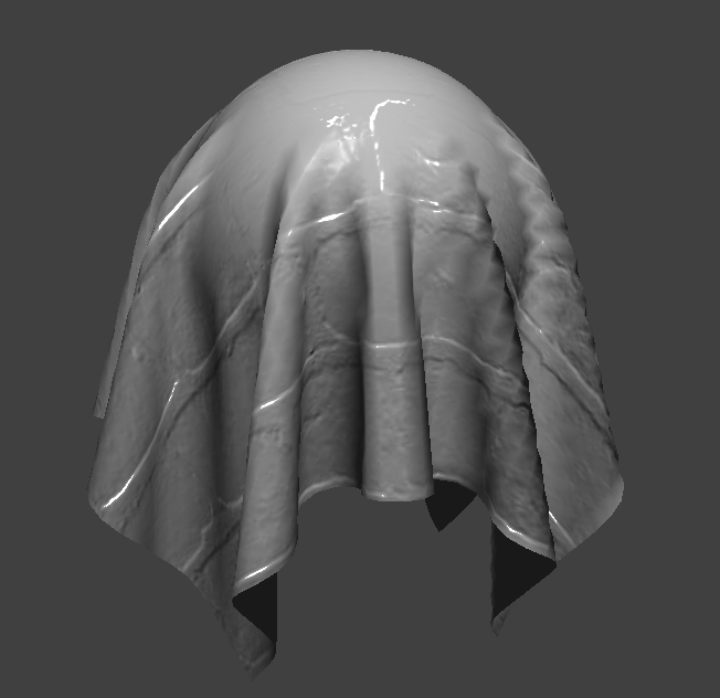
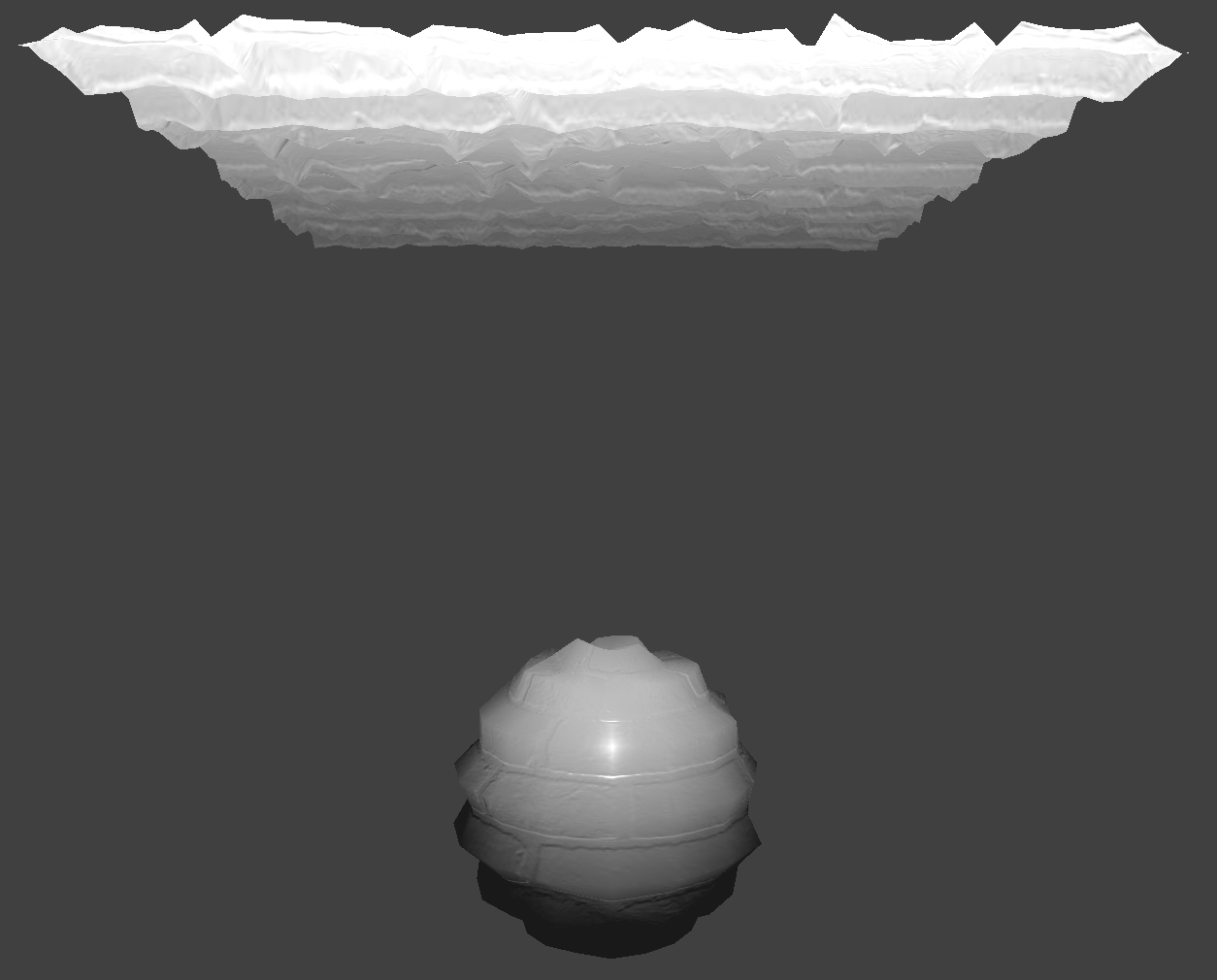
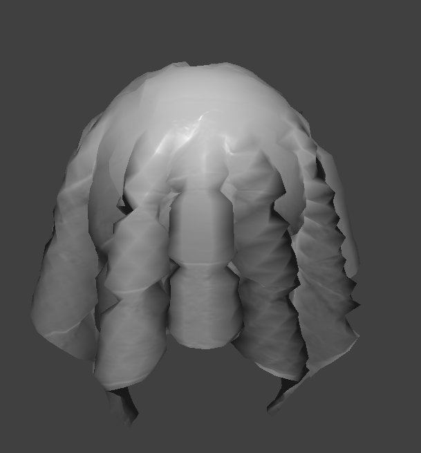
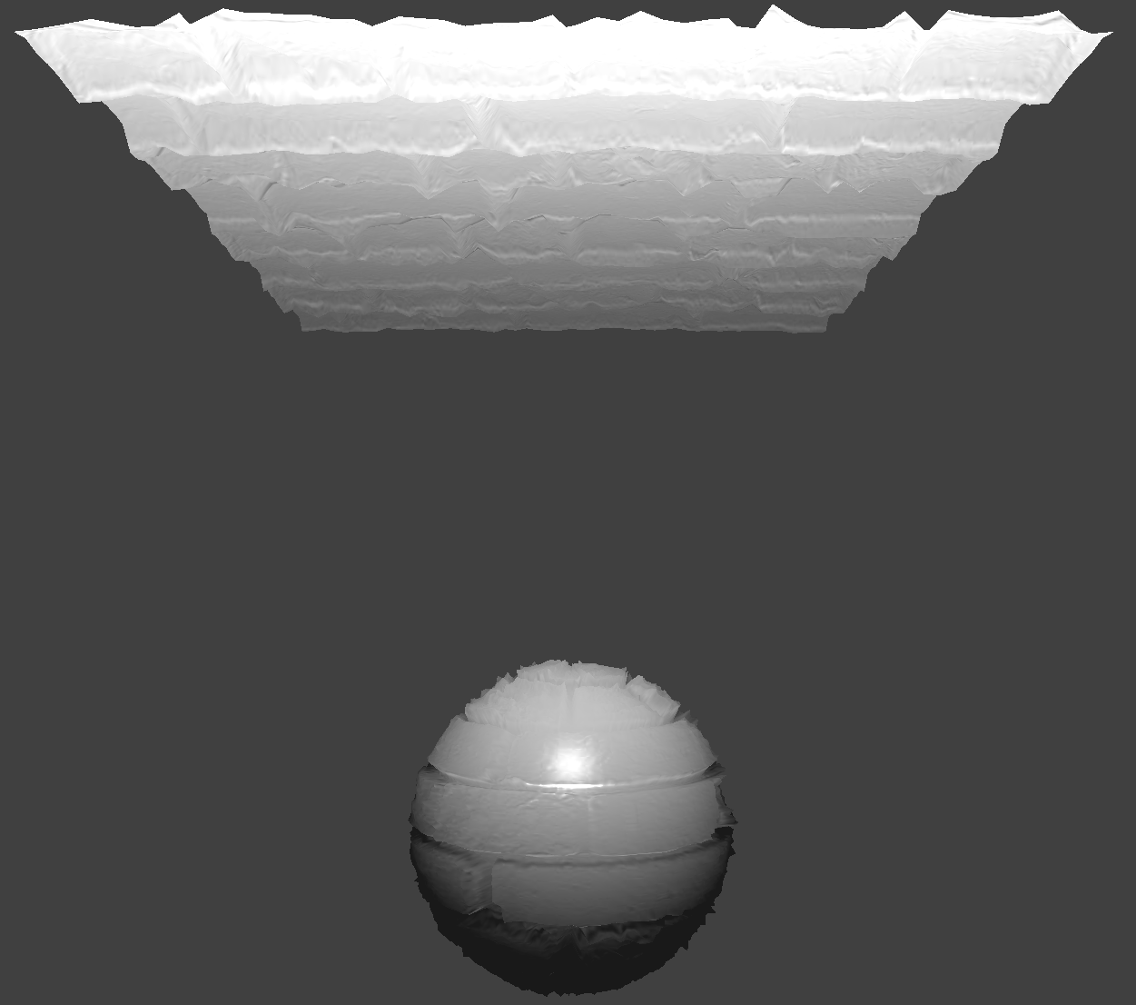
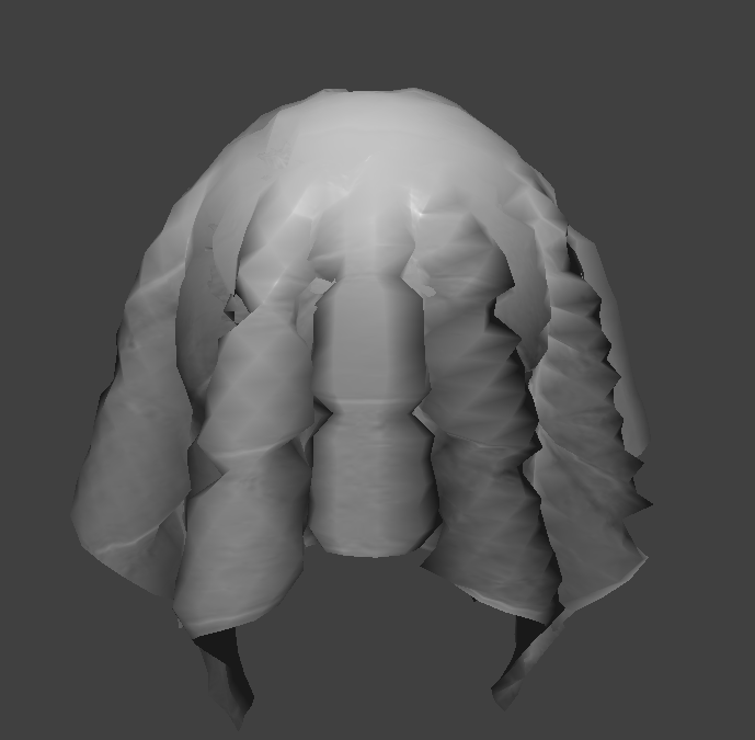
Bump and Displacement Shading
Rendering an image with bump mapping as compared to displacement mapping changes how the resulting renders look. Bump mapping causes little to no impact on the shape of the sphere. On the other hand, displacement mapping significantly alters the silhouette of the sphere. The vertices of the sphere and cloth seem to be more spread apart.
Here are images of the Bump Mapping Shader:
|
|
Here are images of the Displacement Mapping Shader:
Using texture3.png!
|

|
16 Coarseness vs 128 Coarseness
When we use a low coarseness of 16, there seems to be no difference between both approaches. When we use a higher coarseness of 128, the displacement map is a lot more accurate. The sharp edges correspond to where there should be bumps. The displaced vertices also are placed closer to where they should be.
Effect of changing coarseness using -o 16 -a 16
|
|
|
|
Effect of changing coarseness using -o 128 -a 128
|
|
|
|
Here are images of the Mirror Shader:
|
|