In this project, we implemented multiple aspects of the path tracing algorithm in order to render various scenes with lighting. Path tracing allows us to illuminate images with realistic lighting using ray intersection techniques. The algorithm determines how much of the illuminance from a light source will arrive at the viewpoint camera. We implemented triangle and sphere intersection algorithms which allowed us to figure out if and where a ray would form an intersection. We also constructed Bounding Volume Hierarchy (BVH) boxes to speed up the process of rendering images. A key part of this project is global illumination; we accomplished this using direct and indirect lighting functions. Lastly, we used adaptive sampling to reduce the noise in our rendered images.
Part 1: Ray Generation and Intersection
We start this project by generating rays and seeing how we can intersect them with triangles and spheres. We are able to generate rays by taking normalized image coordinates and converting them into the world space. Rays are generated starting with the image coordinates which are first converted into the camera space, where the rays are generated, and then converted into the world space. Given a normalized image coordinate (x, y), we can map it to the camera space where we know the center, bottom left corner, and top right corner—which are in terms of the field of view angles along the X and Y axis. A ray in the camera space will start at the camera and intersect with the point on the sensor corresponding to (x, y). We then transformed this ray into the world space which includes transforming the origin and direction. In order to convert the ray into the world space, we used the transformation matrix c2w which dictates the direction of the ray. The origin of the ray is simply the position of the camera, pos.
The triangle intersection algorithm involves checking to see if there is an intersection between the ray and given triangle; it also provides the nearest intersection location. The algorithm Triangle::has_intersection(…) just checks to see if there is an intersection or not and returns a Boolean. The second algorithm, Triangle:intersect(…) is what checks for an intersection and reports the nearest intersection point. Our ray is parameterized by r(t) = O + tD for 0<= t < inf. If we have a triangle with the coordinates P0, P1, and P2, we can use Barycentric Coordinates to set a point P, where P = (1 – b1 – b2)*P0 + b1*P1 + b2*P2. The intersection of the ray and triangle can then be seen when we set r(t) = P. We used the Moller-Trombore algorithm to solve for t, b1, and b2. Once we perform the intersection of the ray and triangle, we return a Boolean depending on whether or not the intersection exists. If t is within the range [min_t, max_t], we know the intersection exists and we return True. If the intersection exists, we update max_t to t. Otherwise, we return False. We also implemented a ray-sphere intersection algorithm which checks to see if the ray intersects with some given sphere. The overall method is similar to that of the ray-triangle intersection algorithm except the equation for a sphere is different which changes the actual intersection. A sphere is parameterized by its center C and has a set of points P which satisfies (P-C)^2 – R^2 = 0. We solve for the intersection and find that t can essentially be solved using the quadratic formula.
|
|
|
Part 2: Bounding Volume Hierarchy
A Bounding Volume Hierarchy (BVH) is a binary tree where all geometric objects are wrapped in bounding volumes, which makes rendering images much faster. We use BVH for collision detection and ray tracing because it allows us to determine the location of pixels within different objects.
To construct the BVH, we first construct the BBox object by iterating from start iterator to end iterator and expanding the bounding box; then we construct the BVHnode. We also check the number of primitives in the current BVHnode with a size variable, calculated by iterating from the start to end iterator; if the size is less than max_leaf_size, then it means we are at a leaf node and we set the left and right child to null, set the start and end, and return without recursing further. Otherwise, we must recurse using the heuristic to pick the splitting point.
The heuristic chosen was to first find the largest axis by comparing the bounding box’s extent among the three axes. Then we sort the vector of primitives, between “start” and “end,” according to the primitive’s centroid value on the corresponding “largest axis” found in the previous sentence. Then once the vector is sorted we split the sorted vector in two, and recursively call construct_bvh; this is done by setting node->l = construct_bvh(start, midpoint,max_leaf_size) and setting node->r = construct_bvh(midpoint, end, max_leaf_size) where midpoint = (start + size)/2. We set midpoint as the end iterator for the left half, and set midpoint as the start iterator for the right half, which lets us split the vector into two halves at each step. Finally we can return the constructed node. We felt that splitting based on the centroids according to the axis with the largest bounding box extent was the simplest way to fairly split the image into two sections evenly.
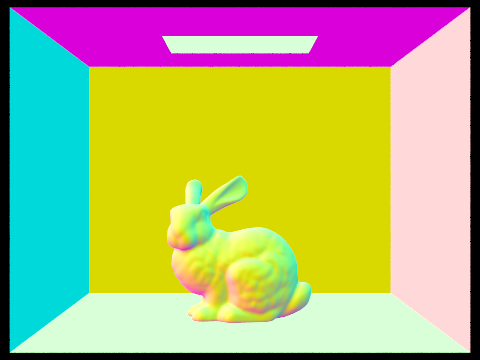
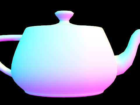
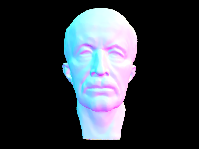
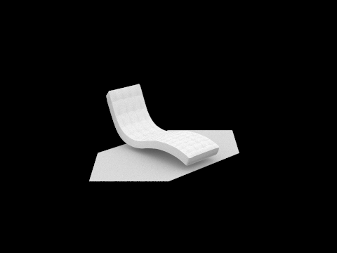
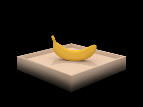
Normal Shading for large .dae files that can only be rendered with BVH Acceleration
|
|
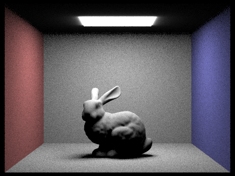
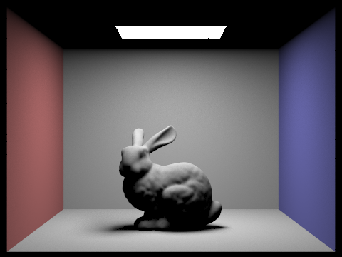
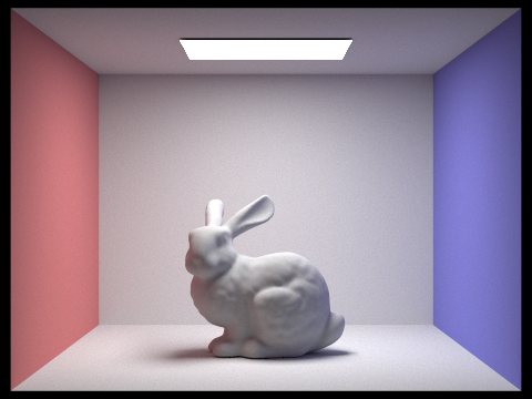
We used the image of a bunny to compare the rendering times with and without BVH acceleration. With BVH, the average speed is roughly 0.3631 million rays per second and we conduct roughly 32.781574 intersection tests per ray. Without BVH, the average speed is roughly 0.004 million rays per second and we conduct roughly 28,588 intersection tests per ray. We can see that rendering images with BVH acceleration is about 90 times faster than not using BVH acceleration. Additionally, BVH acceleration allows us to significantly reduce the number of intersection tests per ray that occur. On average, we conduct 1,180 times more intersection tests per ray when we do not use BVH. This is why our speed is significantly faster when using BVH acceleration.
Comparing the rendering times with and without BVH acceleration for the bunny:
WITH BVH ACCELERATION
./pathtracer.exe -r 480 360 -f bunny.png ../../../dae/sky/CBbunny.dae
[PathTracer] Input scene file: ../../../dae/sky/CBbunny.dae
[PathTracer] Rendering using 1 threads
[PathTracer] Collecting primitives... Done! (0.0136 sec)
[PathTracer] Building BVH from 28588 primitives... Done! (0.2081 sec)
[PathTracer] Rendering... 100%! (0.4758s)
[PathTracer] BVH traced 172800 rays.
[PathTracer] Average speed 0.3631 million rays per second.
[PathTracer] Averaged 32.781574 intersection tests per ray.
[PathTracer] Saving to file: bunny.png... Done!
[PathTracer] Job completed.
WITHOUT BVH ACCELERATION
./pathtracer.exe -r 480 360 -f bunny.png ../../../dae/sky/CBbunny.dae
[PathTracer] Input scene file: ../../../dae/sky/CBbunny.dae
[PathTracer] Rendering using 1 threads
[PathTracer] Collecting primitives... Done! (0.0127 sec)
[PathTracer] Building BVH from 28588 primitives... Done! (0.1483 sec)
[PathTracer] Rendering... 100%! (457.9295s)
[PathTracer] BVH traced 172800 rays.
[PathTracer] Average speed 0.0004 million rays per second.
[PathTracer] Averaged 28588.000000 intersection tests per ray.
[PathTracer] Saving to file: bunny.png... Done!
[PathTracer] Job completed.
Part 3: Direct Illumination
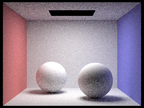
We implemented two different direct lighting functions: direct lighting with uniform hemisphere sampling and direct lighting by importance sampling lights. In direct lighting with uniform hemisphere sampling, we sample uniformly from the hemisphere and estimate the intersection coming directly from the light. In our method, we sampled the light coming into the point w_in and converted those rays to world space using our transformation matrix o2w. We then created a new intersect struct and shadow ray such that the origin is at the hit point and the direction is wi_world. If the shadow has an intersection at any point, we calculate fr using intersection’s bsdf from w_out and w_in, and use get_emission(), multiply these values together with cos_theta(w_in), and we add this value to L_out. And at the end we must normalize & average by dividing L_out by the pdf (which is 1.0/(2.0*PI) for hemisphere sampling) and the number of samples before returning.
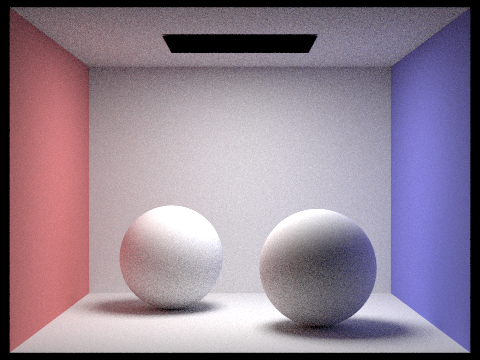
In direct lighting by importance sampling, our goal is to increase efficiency by sampling from the light source directly. We iterate through the light sources; if it’s a point light source num_samples = 1 otherwise the number of samples is ns_area_light. We then iterate “num_samples” number of times. Within each iteration, we first call SceneLight::sample_L() which takes a hit point and returns the incoming radiance and populates wi, distToLight, and pdf. If cos_theta of wi transformed to object coordinates is greater than or equal to 0, then we also create a new shadow ray with the origin being the point and direction being wi. It’s important to set the ray’s min_t to EPS_F and max_t to distToLight - EPS_f to have proper intersection checks. If the shadow ray does not intersect anything, then we will set a temp vector to radiance*fr*cos_theta(wi in object coords) and divide that by the pdf due to the light sampling distribution bias. We must also average L_out by the number of samples for each light source. We then return Lout which is the light that is outputted.
|

|
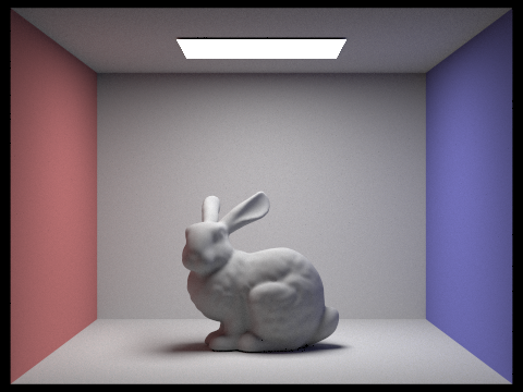
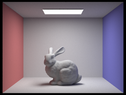
We can see some difference between the images where we used uniform hemisphere sampling as compared to lighting sampling. The image with uniform hemisphere sampling has a lot more noise overall. We can see this on the bunny as well as the background. The image with lightning sampling has significantly less noise and is more smooth. Between the two images, you can also notice that the light source at the top for uniform hemisphere sampling is a bit blurred on the sides whereas we do not see that in lighting sampling. The edges of the room in the image with lighting sampling are also a lot more precise.
|

|

|
|
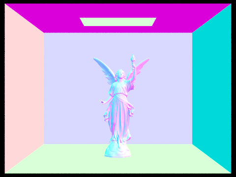
Part 4: Global Illumination
The indirect lighting function allows us to render images with global illumination, in combination with direct lighting which we implemented earlier. We utilize Russian Roulette in order to provide an unbiased estimate; currently, setting a maximum depth leads to a biased estimate which is what we are trying to avoid. We use the function est_radiance_global_illumination() which estimates the total radiance given some direction. We use zero_bounce_radiance, one_bounce_radiance, and at_least_one_bounce_radiance to return the light resulting from zero bounces, direct illumination, and indirect illumination, respectively.
In this section, we focused on implementing at_least_one_bounce_radiance which is what gives us indirect illumination. To do that, we set a termination probability between 0.3 and 0.4 which we use later when determining whether or not we want to terminate the recursive call. Conditions for terminating include coin_flip(termination probability) to be true or reaching the maximum depth. Otherwise, we calculate a new ray with origin and direction calculated via w_in, o2w * w_in, and hit_p, and EPS_F, and one less depth value to keep track of how many times we have recursed; if there is an intersection between the new ray and bvh, then we recurse by calling at_least_one_bounce_radiation with the new ray and eventually add this value to L_out via L_out += (w_in.z * reflectance * recurse)/pdf/(continuation probability). We also need to ensure that there is at least one indirect ray intersection which is why we check if r.depth == max_ray_depth and subsequently recurse by calling at_least_one_bounce_radiance (repeating the process that was described in the above sentence).
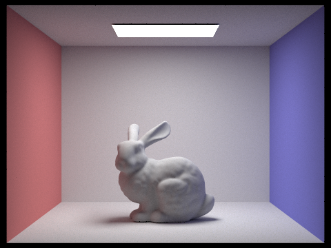
Images with Global Illumination:
|
|
Bunny Images with various max_ray_depth values:
|
|
|
|
|
Images with only direct and only indirect illumination:
|
|
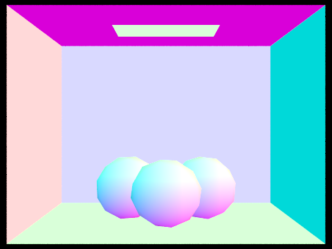
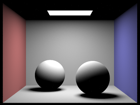
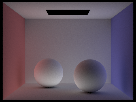
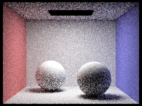
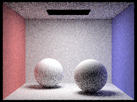
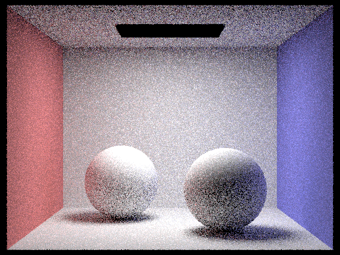
Spheres with various sample-per-pixel rates:
|
|
|
|

|
|
|
|
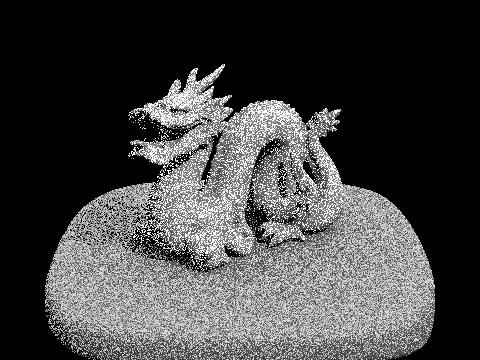
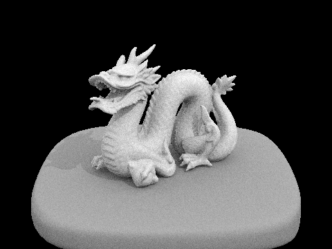
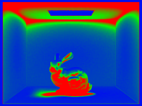
Part 5: Adaptive Sampling
In this last part, we implemented adaptive sampling in order to reduce the noise that’s visible in images. We know that some pixels converge faster than others depending on the sampling rate. Adaptive sampling uses a large, fixed number of pixels by concentrating the pixels in the more difficult parts of the image. In our algorithm, we iterate through individual pixels and detect whether or not the pixel has converged. We do this by finding their mean and standard deviation; using the formula I = 1.96 * standard deviation/sqrt(n), we can figure out what the pixel’s convergence is. When I < maxTolerance * mean, we stop tracing more rays for that pixel. Additionally, to avoid checking a pixel’s convergence for each new sample (which can be very costly), we use samplesPerBatch so that you only need to check whether a pixel has converged every samplesPerBatch pixels.
|
|