path tracer

Nadia Hyder, CS 184 Spring 2021

 

 

OVERVIEW

In this project, I explored and implemented several path tracing algorithms to render images with realistic, physical lighting. This project consists of 5 parts: ray generation and scene intersection, bounding volume hierarchy, direct illumination, global illumination, and adaptive sampling. 

 

 

TASK 1: RAY GENERATION AND SCENE INTERSECTION

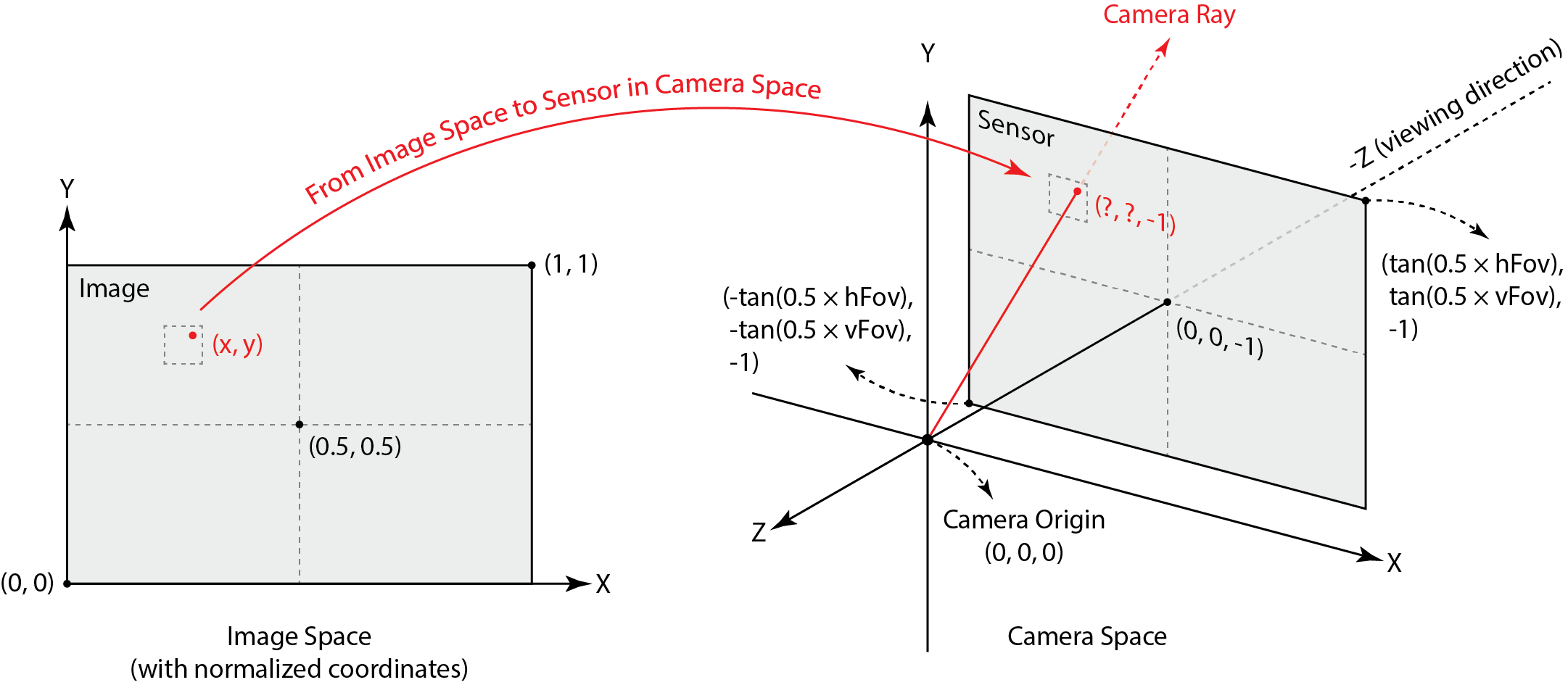
I first generated camera rays, taking normalized image (x,y) coordinates and outputting them as Ray objects in the world space. In order to do so, I first transformed the image coordinates to camera space coordinates, generated rays in the camera space, and finally transformed them into a Ray object in the world space, characterized by an origin and direction.

The image below shows mappings from the image space to the camera space. 

 

To determine when and where a ray hits an object, I wrote the Moller-Trumbore algorithm for ray-triangle intersections:

 

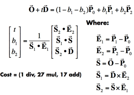
This algorithm both gives us the time, t of intersection and allows us to express an intersection point in terms of barycentric coordinates, used to perform a point-in-triangle test. If t is within the ray’s minimum and maximum possible time and the intersection points are between 0 and 1, and valid intersection has occurred. I then store t, the surface normal at the intersection, the primitive type (triangle in this case) and the bsdf value in an Intersection object.

 

With ray tracing and scene intersection, I was able to generate images with normal shading:

 

 

 

 

TASK 2: BOUNDING VOLUME HIERARCHY

Next, I implemented a bounding volume hierarchy binary tree. Nodes in the tree represent a subset of primitives in the scene. An internal node stores a bounding box of all objects inside it and reference to child nodes, while a leaf node stores its bounding box and a list of objects. The BVH allows us to quickly traverse the scene and quickly discard primitives that a given ray will not intersect. Next, I implemented a method to split the tree. For each bounding box axis, I computed the mean of the centroid, and traversed all primitives in the axis, placing bboxes with centroids greater than the mean in a right tree, and others in a left subtree. I split across the axis with the smallest heuristic cost, calculated by summing the product of the extent of the box over every axis. I recursed and split the tree further into right and left bounding boxes based on centroid values.

Using BVH acceleration I was able to efficiently render images with several thousand primitives in a matter of seconds:

 

 

Using a BVH gave massive speed-ups and performance improvements. I was able to render scenes with many primitives at much faster speeds; without BVH rendering the cow took 2 minutes and 31 seconds, and I could not even render maxplanck or CBlucy on my machine. BVH improved the speed greatly by discarding nodes with bounding boxes and primitives that do not intersect with the camera rays. I was able to reduce the run time from O(n) to O(log n), where n is the number of primitives in the scene.

 

As a side note, the intersection tests make a huge difference in performance. On my first attempt, my triangle intersection test was buggy and rendering cow.dae took 31 seconds.

 

 

 

 

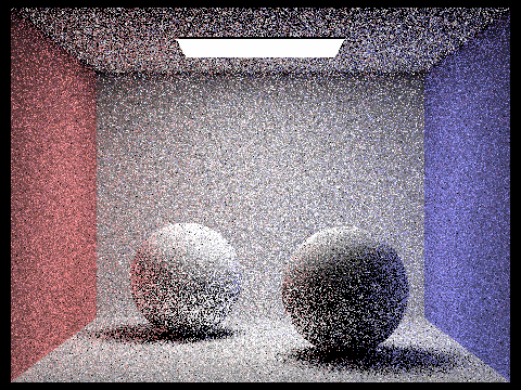
TASK 3: DIRECT ILLUMINATION

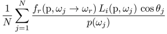
For the next part of the project, I simulated light transport in the scene to render images with realistic shading. I implemented two direct lighting estimation methods: uniform hemisphere sampling and importance sampling. I then used Monte Carlo integration to estimate irradiance.

 

To perform uniform hemisphere sampling, I estimated the direct lighting on a point by sampling in a hemisphere uniformly. I first converted the hemisphere to world coordinates and calculated a ray with the sample as the direction and (sample + point of interest) as the origin. If the ray intersected the BVH, I computed the amount of light arriving at the intersection point using a Monte Carlo estimator. The Monte Carlo estimator integrates over all light arriving in a hemisphere around a point of interest:

The following is the result of running uniform hemisphere sampling for CBspheres_lambertian.dae:

 

 

 

 

To perform importance sampling, I sampled all light directly rather than over uniform distributions in a hemisphere. This performed better than uniform hemisphere sampling, which was quite noisy. I summed over every light source in a scene and sampled directions between the light source and the point of interest, hit_p. Like in the previous part, I checked if the cosine of the ray was positive (the light is in front of the object and visible) and if it intersected the BVH. I then Monte Carlo integration. If the light was a delta light, I only sampled once, as all samples would be the same.

This is the output from importance sampling for CBspheres_lambertian.dae:

 

When there are fewer light rays, the rendered images are noisier. The images below show outputs from rendering with increasing numbers of light rays and 1 sample per pixel using importance sampling: As the number of light rays increases, shadows are more visible and the images are less noisy due to having enough light rays to match the amount of information. Increasing the number of light rays and samples gives more realistic images.

 

To conclude this section, the two images below show how an image is rendered using uniform hemisphere sampling and how the same image is rendered using importance sampling. We can see how the two approaches generate very different results; uniform sampling gives us a much grainier, noisier image, This is because we only sample the hemisphere and miss several rays, yielding a darker image with several dark spots. Importance sampling, however, effectively considers rays that influence the result by sampling lights. Importance sampling uses more information (and thus better represents information) but is more time and resource intensive.

 

 

 

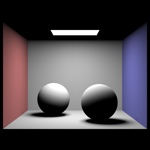
TASK 4: GLOBAL ILLUMINATION

In task 3, we only looked at direct lighting. In this part, I took it a step further and considered full global illumination to render the effects of indirect lighting.

To implement this, I found the radiance when there are 0 bounces of light () and 1 bounce of light. I could then find the radiance when there is at least one bounce of light (in the function at_least_one_bounce_radiance) by using the summing zero_bounce_radiance with at_least_one_bounce_radiance, which sums its radiance with one_bounce_radiance over several recursive calls. at_least_one_bounce_radiance traces a ray in the direction of a given sample based on the BSDF at the hit point, and recursively calls itself on the new hit point. While the goal in this part is to integrate over as many paths of all lengths, we cannot realistically perform this, so I used Russian Roulette for an unbiased method of random termination. Termination probability can be arbitrary; I used a termination probability of 0.3. I recursed until reaching the maximum number of ray bounces (max_ray_depth) or until the new ray no longer intersected the BVH (the ray does not bounce off anything).

 

Here is a comparison of the same image rendered with different lighting:

 

The following gif of bunny.dae shows how the image changes with increasing ray depth. The images are rendered with max_ray_depth of 0, 1, 2, 3, and 100 with 1024 samples per pixel:

 

 

 

 

 

 

 This gif shows the effect of increasing sample-per-pixel rates for spheres.dae. Sample rates are 1, 2, 4, 8, 16, 64, and 1024 with 4 light rays:

.

 

 

TASK 5: ADAPTIVE SAMPLING

For the final part of this project, I implemented an algorithm for adaptive sampling. Monte Carlo path tracing produces noice due to the large number of samples per pixel. Adaptive sampling is used to reduce the number of samples per pixel by determining which pixels need more samples to get rid of noise and which converge faster. This algorithm calculates a 95% confidence interval of μ – I and μ + I. I solved for pixel convergence I:

I is small when the samples variance is small, so when I <= maxTolerance * μ,  we assume the pixel has converged and do not trace anymore rays for the pixel.

 

I calculated the mean and variance as follows:

 

 

After implementing adaptive sampling, this is what bunny.dae and its sampling rate image look like, with 2048 samples per pixel and max ray depth of 5: