CS 184: Project 1

Overview

This project is about the partial implementation of a svg-format graphics rasterizer, which incorporates basic concepts such as triangle rasterization, antialiasing via supersampling, and texture mapping in the first two weeks of the course.

Overall, the focus centers around three core functionalities for rendering triangles with simple color, interpolated colors, and external texture. In the first two cases the goal is to develop efficient algorithm that calculate pixels within the triangle and fill them with color provided or interpolated using barycentric coordinates. Antialiasing is achieved through supersampling and then downsampling with box filter (average).

After that, much time is spent on the last part rendering textured triangles. The mapping from xy screen space to the uv texture space once again depends on barycentric coordinates; for texture sampling, two methods sample_nearest and sample_linear are implemented in addition to three ways (L_ZERO, L_NEAREST, L_LINEAR) of determining the mipmap used for each pixel in the screen space.

This is my first time writing a large project with C++, and it's exciting to see how its wordy syntax and static typing trade off with super fast execution speed (e.g. v.s. vanilla Python). Putting textbook/slides knowledge and algorithms into actual codes requires taking care of many engineering details and edge cases, but it's exactly such sophistication in implementation that brought me sense of fulfillment after finishing everything.

The only regret is that other interesting parts of a functional svg renderer, e.g. parser and svg element objects, are given in the skeleton code. This is reasonable since this course is about graphics, not software engineering or compiler. If I have more time, I would love to add support for more svg elements such as Path.

Task 1: Drawing Single-Color Triangles

Steps for rasterizing a single-color triangle

Since the order of the given triangle vertices are not guaranteed, the first thing I did is to reorder the vertices in a consistent manner so that downstream codes don't need to handle different cases separately. I chose to adopt the counter-clockwise order. What I did is to first find the rightmost vertex (with largest x value, denote as p2), and then find and compare the two slopes between this vertex and the other two (the other vertex with lower slope is denoted p0, and p1 for the last one). Then I did a in-place reorder using swap function and the above algorithm returns the vertices in desired order.
The second step is just the straight-forward pixel in triangle test mentioned in lecture. Some technical details that helps optimize the speed include precomputing the normal vector for each triangle edge and setting up a bounding box using the min/max values of x/y coords. I also stored the line distances (i.e. dot product between edge normal and the vector from vertex to test point) in local variables for computing barycentric coordinates (mention later).
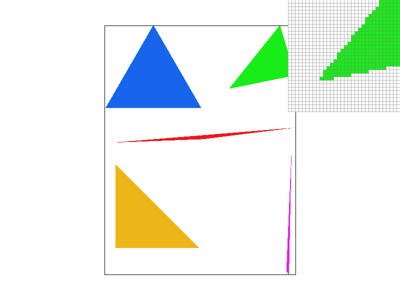
Once a pixel is deemed as within the triangle, I use the floor function to determine its indices in the frame buffer (make sure the indices are valid) and call rasterize_point (later changed to fill_pixel) to draw it.
When the above is finished, we can successfully render svg such as the one below:

basic/test4.png

Task 2: Antialiasing by Supersampling

Overview

The vanilla triangle rasterization in the last section assigns binary color to each pixel (either colored or white) and there's no in between. Naturally this gives rise to jaggies and sharpness in the border which are parts of aliasing. To overcome this, the core idea is to enable the pixels to take intermediate colors by sampling more frequently (supersampling) and then downsampling (average) so that the image size remains.

Steps and Modifications

Supersampling by definition is to break each pixel in the screen space into n sub-pixels (n usually square of some integer) and perform the pixel in triangle test above at these sub-pixel level. But on the other hand, we can also think of it as having a larger screen space sqrt(n) * width x sqrt(n) * height and apply the method in Task 1 on a larger scale. To achieve this, we need to equivalently scale up the triangle vertices by sqrt(n). Since the larger screen space is different from the frame buffer we want to display, now the pixels are firstly drawn to the supersample_buffer for further processing. This requires modifying the fill_pixel method so that it no longer writes to the frame buffer (I didn't follow the hint to implement fill_supersample so the rasterization of point, line, triangle shares the same fill method).
With the supersample buffer filled up successfully, we need to perform downsampling to output graphics of correct shape and achieve antialiasing effect. This is handled by the resolve_to_framebuffer method which is called lastly in DrawRend::redraw. The implemention is straight-forward since we are simply doing an convolution with kernel size sqrt(n). The only technical issue that somewhat bothered me is the conversion of indices from supersample buffer to the actual buffer since they are using different representations. The color class provided by CGL has overloaded arithmatic operations which makes it really easy to work on them.
Lastly, with the introduction of a new buffer and varying parameter sample_rate, I implemented utility functions such as clear_buffers, set_framebuffer_target, and set_sample_rate. These methods are trivial for someone familiar with OOP.

sample rate = 1

sample rate = 4

sample rate = 16

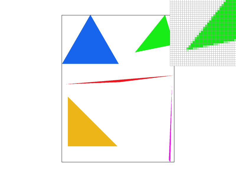
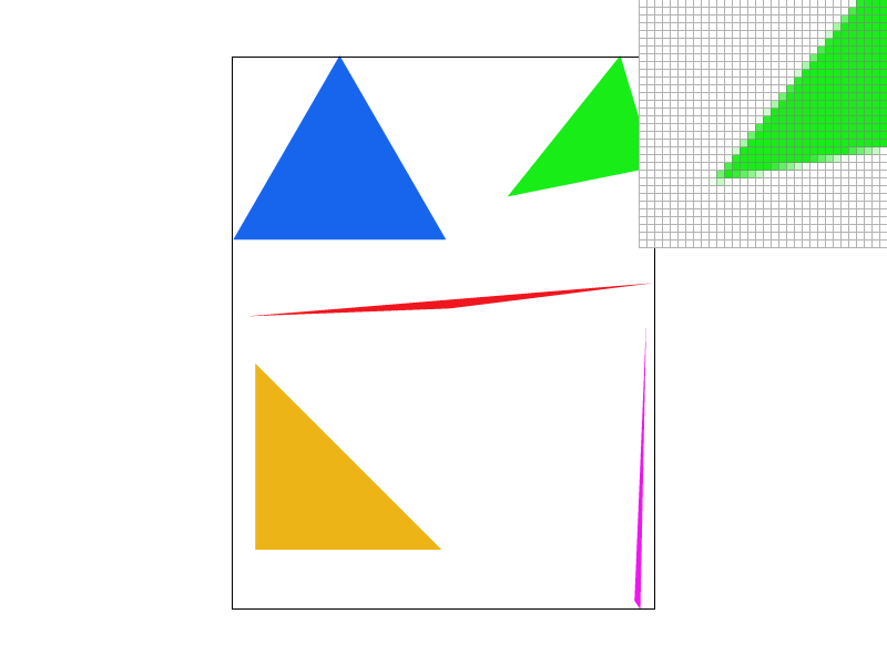
As we can see from above, as the sampling rate increases, the border pixels of the triangle (see inspector) takes more variety of values and the entire image looks more smoother (the difference between 4 and 16 case is not so obvious since test4.svg is a relatively simple one). Many pixels around the green triangle which are white in the original case takes on light green values as a result of supersampling. As a result the jaggies get reduced tremendously as the sudden change of color is replaced by a gradual development.

Task 3: Transforms

robot playing soccer

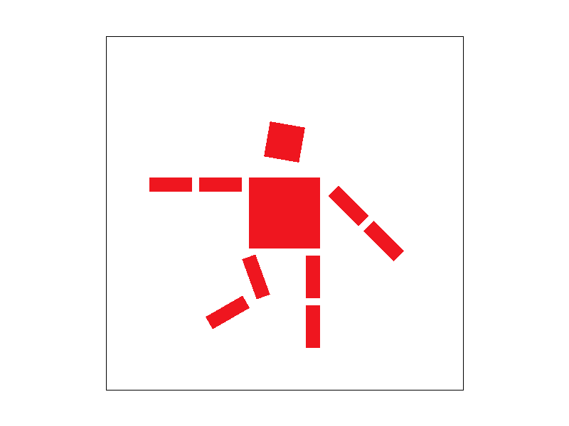
Additional rotations and translations are added so that the robot looks like playing soccer and about to shoot for a goal.

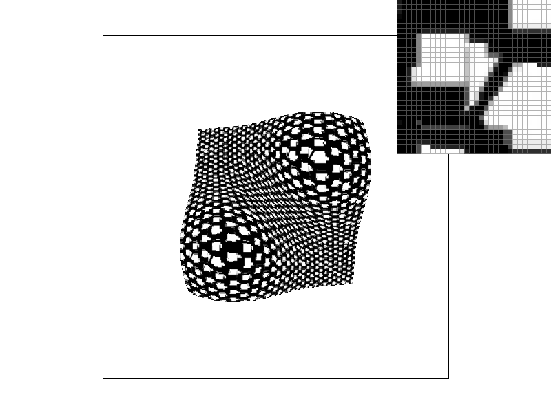
Task 4: Barycentric coordinates

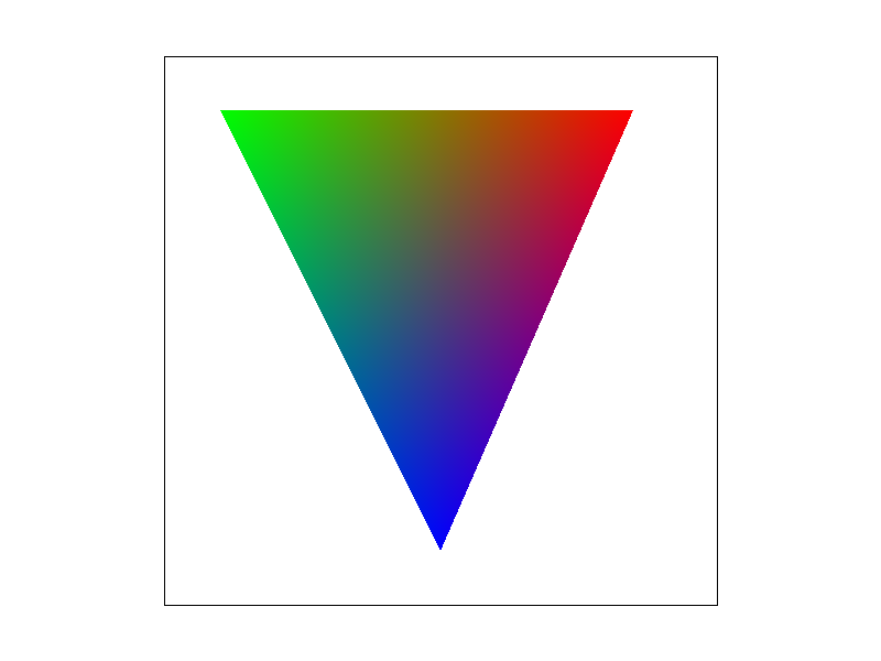
Barycentric coordinates provides a basis (coordinate system) to uniquely describe each point within a triangle using the three vertices. To be more precise, the attribute (including but not limited to location, texture space coordinates, color) of each point can be expressed as a linear combination of the attributes of the three vertices, with the additional constraint that the weights of linear combination sum to 1 (and positive since within triangle). The graph on the image is an example of using barycentric coordinates to interpolate triangle colors given the colors in the three vertices (R, G, B respectively). For each point inside, the closer it is to one of the vertex (say green vertex on the left), the closer its color to that vertex's color (greener). This results in the entire graph being blended color triangle.

Task 5: "Pixel sampling" for texture mapping

Pixel sampling is the process of getting color from the texture image (uv space) corresponding to the query point (u, v), which are usually calculated using aforementioned barycentric coordinates in the screen space (xy space). The obtained color are used for texturing the output image as we have done in coloring the triangles.

Nearest Sampling: this is the sampling method that returns the color of the nearest pixel in the texture. In actual implementation, this method only requires taking the floor of the u\v coordinates and then extract the actual color at that pixel with Mipmap::get_texel.
Bilinear Sampling: bilinear sampling can be thought of the extension of linear interpolation to the 2D case. In the 1D case, two points uniquely determine a line and we can find the interpolated values (y values) corresponding to other x values on it. In binlinear sampling, we firstly try to find the four pixels that "surround" our query point (whose centers form a square that contains the point), then we separately interpolates the upper/lower two pixels using the horizontal distance from the query's x coordinate to the left, and finally interpolate again using its vertical distance from above. In the actual implementation, I utilize round instead of floor function to get the center x/y position of the aforementioned "surrounding square", so that round(x) and round(x - 1) corresponds to the left and right pixel locations (similar for y). Finally, we implement the lerp function to help with interpolating the color as described above.

There are certain edge cases for bilinear sampling. For example, if the query point is close to the rightmost edge of the texture image, it's impossible to find all 4 sample locations as mentioned before. My implementation uses nearest sampling to handle such scenario.

nearest sampling, sample rate = 1

bilinear sampling, sample rate = 1

nearest sampling, sample rate = 16

bilinear sampling, sample rate = 16

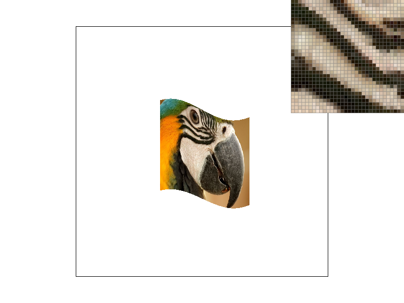
The difference between these two methods are best illustrated when there are abrupt change of colors in a certain part. In the above examples, the inspected region displays the alternating stripes around the parrot's eyes. We see that, with the same sample rate, bilinear method gives smoother gradient transition effect from one color stripe to another, while the nearest method looks sharper. This looks similar to the effect of increasing sample rate. It's not hard at all to explain this phenomenon since the bilinear sampling tries to integrate color information from neighboring pixels as well, which is exactly what we do when in supersampling (the difference is that supersampling is followed by averaging, but here bilinear interpolation is used).

Task 6: "Level sampling" with mipmaps for texture mapping

Level sampling is the process of finding the appropriate level of mipmap for each pixel based on estimating its screen pixel footprint in texture. Intuitively, from these slides we see that using a high level mipmap across pixel will make closer regions too blurry while using a low level one causes jaggies for further scenes. So a computed, adaptive algorithm for finding mipmap level is needed.

To implement level sampling, we need to obtain the uv coordinates of (x, y + 1) and (x + 1, y) for each point (x, y) in the screen space. This unavoidably leads to redundant computation if the original rasterize_textured_triangle method is used. So I add a HashMap for caching purpose. Once this step is done, the required parameters are wrapped into a SampleParams object and passed to Texture::sample, which then calls Texture::get_level to return a continuous level value based on the formula mentioned in lecture. For nearest level sampling, this continuous level is directly rounded; for linear level sampling, an additional interpolation of the results returned by two consecutive mipmaps is appplied. The edge case I encountered is getting some level value too small (< 0). Level 0 mipmap is then used in this case.

Performance Tradeoff:

generally speaking, increasing sample rate will linearly increase the memory usage and running time, while giving better antialiasing effect. For pixel sampling, bilinear sampling is also more costly in time than nearest sampling but also increases antialiasing power as described above. For level sampling, the zero sampling doesn't require any computation at all, and linear sampling is slower than nearest sampling. But the later two methods allows additional degrees of freedom using different mipmaps for different pixels, so the blurring/jaggie issues are better solved.