|

|
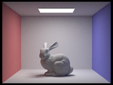
Overall, the project was a lot of work! Most of my implementations were based on the solutions given in lecture or on the spec. Notable parts include my probably not original and likely inefficient but still cool BVH splitting heuristic. Rendering the images for part 4 kind of took a criminal amount of time. I wouldn't surprised if this project was sponsored by intel trying to sell us more CPUs or something; "Falling behind on your project? Well for the small price of $699 you can buy our new core i9 16900k and render your images 3-5% faster!". My suggestions for future iterations is to add hardware acceleration of some sort and let people use their GPUs to render. Like we are CS majors of course we use a 4090 just to be silver in league. Overall, everything else is pretty much normal. I like how now I actually understand what's going on when I render a scene with my 3 free assets in Daz studio and why it still looks grainy after 8 hours of rendering. But I think I've stared at computer generated bunnies for just about long enough now. Maybe in the future you guys can switch it to a cat or something.
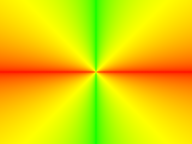
To generate camera rays, I first prepare to conver the pixel from image space to camera space by calculating the maximum X and Y values of the camera space, in other words, the coordinates of the top right corder. Then, I multiply these coordinates by the given X and Y coordinates and by 2. This makes it so that the coordinates are now the correct camera coordinates, except they are shifted to be centered at 1/2 the max camera coordinates instead of at (0,0). To re-center the coordinates, I just subtract it by the maxx and maxy values computed in the first step (where the top right corner is supposed to be). Then, I make a new vector with these x and y coordinates and a z coordinate of -1, convert it to world space, and normalize it. The returned ray has this vector as the direction vector and the camera's position as the origin vector. I also set the min and max t values of the new ray.
To sample pixels, I just sample num_sample times and average the samples for each pixel. This was changed in part 5.
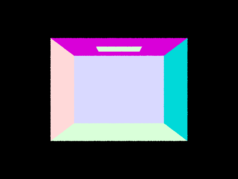
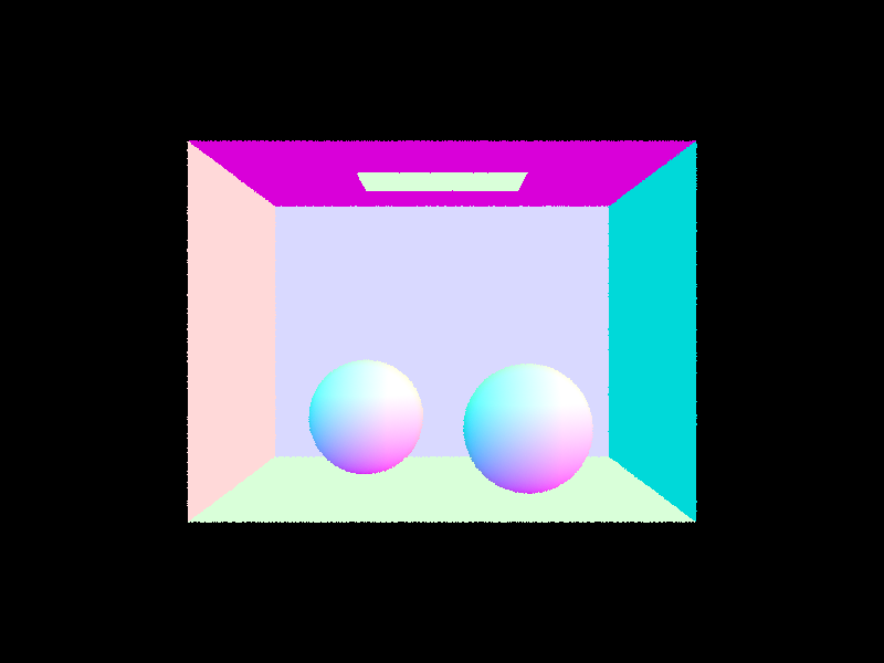
To determine if a ray intersects with a triangle, I used the fancy Moller Trumbore Algorithm from the ray tracing slides which can be found here . This algorithm is more efficient and honestly easier to implement than checking if a ray intersects with the triangle's plane and then checking if it intersects with the triangle. My implementation basically follows this algorithm exactly, even with the exact same variable names as the ones they use in the slides. In has_intersection(), I simply return whether t, b1 and b2 (the barycentric coordinates) are nonzero and if b1 + b2 are less than 1 (so if they are valid barycentric coordinates). In intersect(), the t value is already given in the result vector so no calculation is needed there. Using the b1 and b2, I calculate the normal vector of the intersection. Then, I set isect.primitive and isect.bsdf and we are done. One additional check for both functions is if the resulting t value of the intersection is within the min and max t values of the ray.
|
|
|
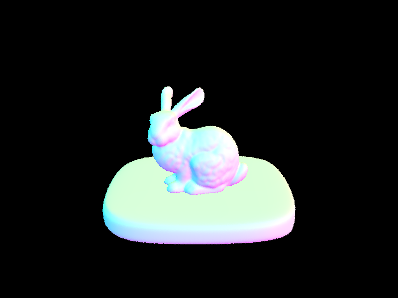
|
My idea for constructing the BVH was to split each node on the plane where the positions of the primitives have the highest range, AKA the largest difference between their lowest and highest value. After choosing x, y or z, the line to split the plane would be drawn at the mean of the positions of the objects in that coordinate. So for example, if x was the chosen plane to split, then everything above the mean x would be in one new node and everything below the mean x would be in another new node. To do this, I had to keep track of the min and max x, y and z values, as well as the sum of the x, y and z values of every primitive while looping through them. I also expand a bounding box around everything, so if the current box is to be a leaf node, then I can just return that box. Otherwise, I then find out which axis has the largest range, calculate the mean value for that axis, and partition the primitives based on that. I would have to loop through everything again to partition, but luckily std has a partition() function for exactly this purpose. Using the computed axis and mean, I can ensure that partition returns the iterator position for the midpoint, and I can just use this, along with the start and end iterators, to pass into the recursive call for constructing the child nodes. This partition function was a real lifesaver, because not only is it probably faster than looping through everything and creating new iterators, I was also running into segfault issues where I would create a new vector and iterators for the recursive calls, but they would somehow get destroyed along the way as a recursive call would returns. For an additional base case, if the midpoint iterator was somehow the same as the start or end iterators, in other words eveyrthing got partitioned to one side of the mean, then I would just treat that node as a child. This shouldn't be possible unless all the nodes have the exact same position in every axis (since I choose the axis with the largest range). In this case, splitting the bvh into more children nodes wouldn't speed anything up and would instead slow down ray tracing as the ray needs to traverse the BVH tree for longer. So overall, I am pretty proud of my little bvh function. Though there probably better ways to choose the plane to split, my implementation overall splits the primitives pretty evenly and offers substantial speedup.
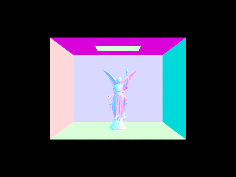
|
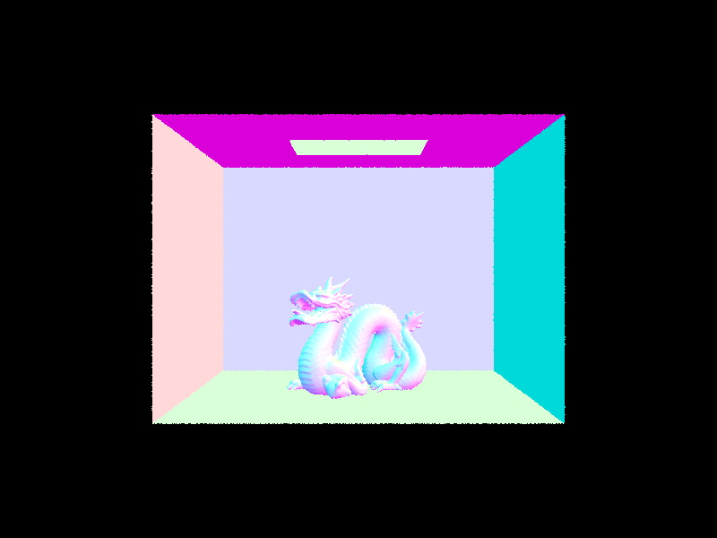
|
|
|
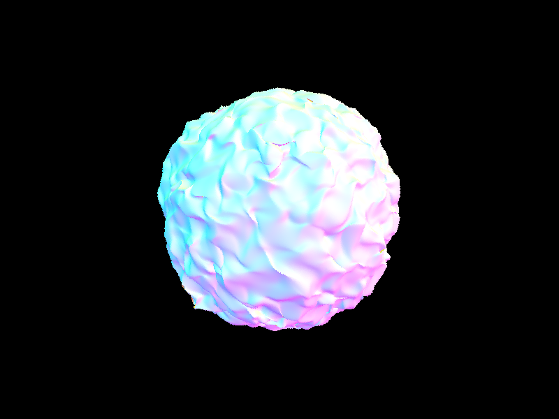
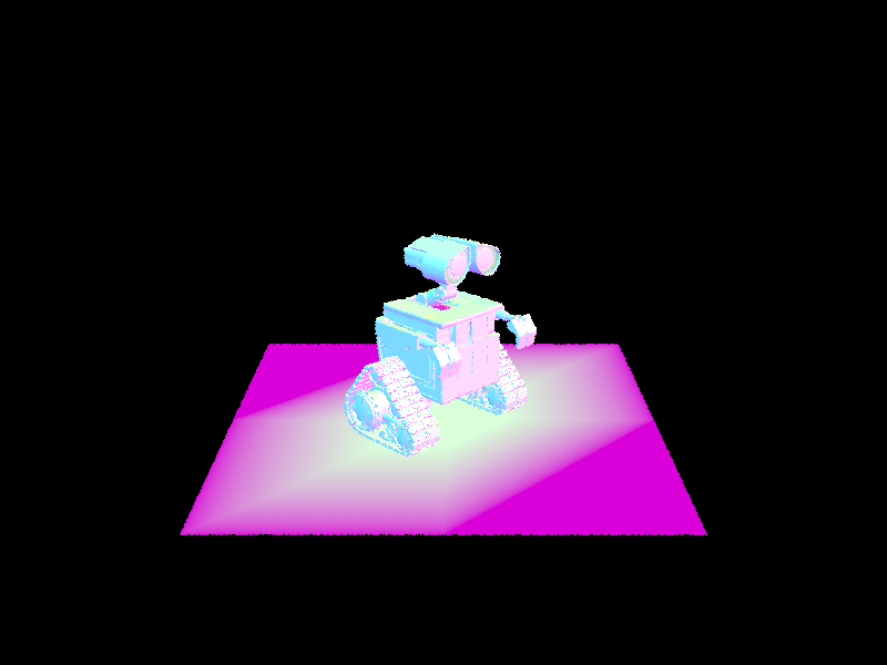
Looking more closely at Blob, rendering blob.dae on one thread with normal shading as above took 0.657 seconds. To see what happens when we don't have BVH acceleration, I made it so that everything is put into one giant BVH leaf node. Rendering Blob again took... and I am not joking when I say that I could have taken a shower a dump and a nap before this thing finished, because it took a whooping 865 seconds to render. That's almost 15 minutes of 100 percent CPU usage on one thread. That's almost as long as it took my dad to come home with the milk. It really just goes to show how much time you can save by not computing the ray intersection for every triangle for every ray in a scene with lots of triangles. I know for a fact that we wouldn't have 60fps Cyberpunk if BVHs weren't a thing. We probably wouldn't even have 60fps Peppa Pig without BVHs. God bless BVHs.

|

|
For zero bounce, we just return the emission from a given point, since only emitted light shows up here.
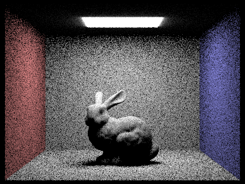
For uniform hemisphere sampling, I began by grabbing a random sample for wi using UniformHemisphereSampler3D. Then, since we are only doing direct lighting, I check if a ray cast in this new direction would hit anything. if not, I skip this sample. Now, we know that we have a ray that hits something. I then compute f, or the color from hitting that intersection from our sampled wi going towards the camera. I also calculate cosine theta, which is the angle between the wi and the normal vector. Cos_theta times f times emission divided by pdf (1/2pi) is then added to L_out. This is done num_sample and the average is returned.
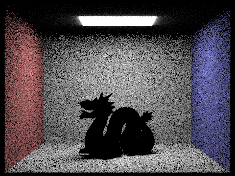
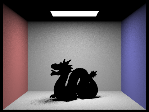
For light importance sampling, I start by looping over the lights in the scene. For each light, I use the light.sample_L() function to sample a random wi direction, as well as get the pdf and emitted radiance from that sample point and direction. I also shoot a new ray towards the sampled wi to check if it intersects with anything, and if it does, then we skip this sample. Otherwise, the rest is the same, where we compute f in the same way as in uniform sampling, and add f times emitted radiance times cosine theta divided by pdf to L_out and average it for all samples taken from that light.
| Uniform Hemisphere Sampling | Light Sampling |
|---|---|
|

|
|
|

|

|
|

|
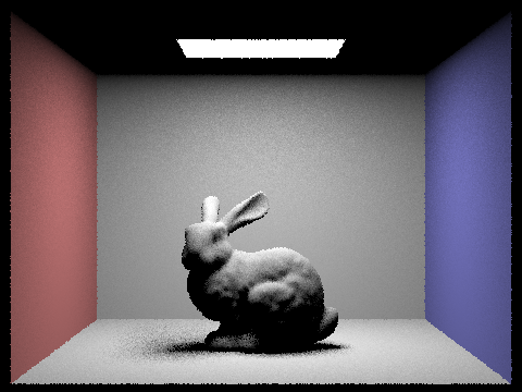
As seen, by increasing the amount of light rays per pixel, the accuracy of the lighting increases. This can be seen the most when looking closely at the bunny's body and the shadow it casts on the ground. The shadows are a lot smoother when using more light rays.
When using the same amount of lighting samples, light importance sampling produces much more realistic and less noisy results. This is because by only sampling in directions where we know lights are, greatly increasing the chance that the rays we shoot out from any given pixel will hit somewhere closer to where the actual light is. When this happens, we can get a more accurate lighting sample for that pixel. When sampling uniformly at random, especially when only using one light sample per pixel, it is quite likely that that light sample comes from like the dark corner or something where there aren't any lights, so as a result the pixel is updated with an inaccurate sample for its color. When using a lot more total samples, both techniques will eventually end up with an accurate image, but importance sampling can achieve a more accurate result much quicker.
To implement indirect lighting, we basically simulate more bounces for a given ray of light. Previously, for direct lighting, from any given pixel we shoot out a ray and see how much light is coming from that direction and bouncing off our pixel and going towards the camera. With indirect lighting, for each pixel, we still keep track of the results from direct lighting. However, now we also sample a new random direction using isect.bsdf.sample_f(), and shooting out a new ray in this direction from the intersection point of the original ray. If this hits nothing we just return the direct lighting for the original point. Otherwise, we recursively call at_least_one_bounce_radiance, the indirect lighting function, with this new ray. Basically, the idea is that we want to find how much light we can see from the new intersection to our pixel, ie our original pixel acts as the new "camera", and we want to know what kind of light we can see from that spot. We add the result times the radiance from sample_f times cosine theta divided by the pdf to our L_out. When adding the recursive result, we also weight it by the continuation probability, since the recursion only goes with the continuation probability chance and up until max_ray_depth times. Some nuances are that if we turn isAccumBounces off, then the function only returns the result of the last bounce rather than adding it along the way.
|
|
|
|
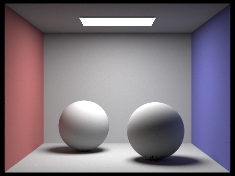
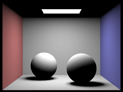
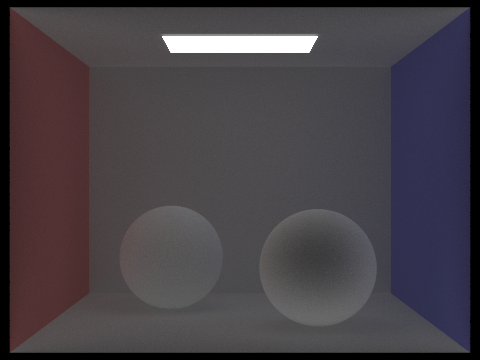
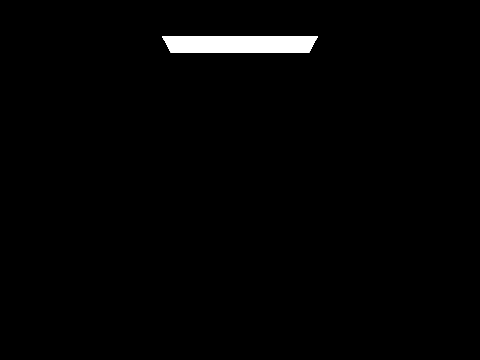
Notice how the only direct illumination has completely black shadows. In places such as the ceiling, where there is no direct line of sight to the light, the pixels are completely black. Now, looking at the only indirect lighting, notice how the colors look a lot more washed because there is no direct lighting. The darker places on the indirect lighting are the places where less indirect light is being reflected, such as onto the right sphere. This differs from the darker places in the direct lighting, as those are where the actual shadows are.
|

|
|

|
|
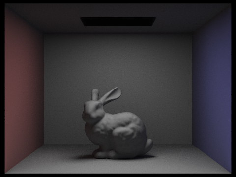
|
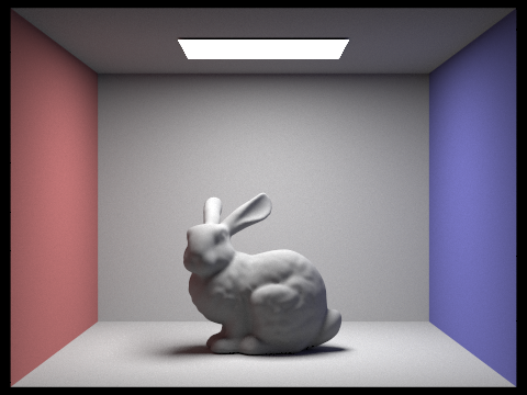
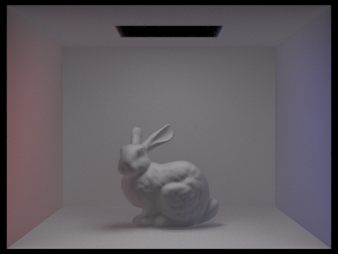
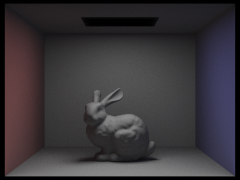
No accumulation for max depths 0 and 1 are the same as with accumulation, because it is just zero bounce and direct lighting. However for 2 bounce onwards, each of the subsequent bounces contributes a little bit of light to the actual image. This amount of color is decreasing however, and the image gets darker and more washed out the more light bounces around since it is being normalized as it is going.
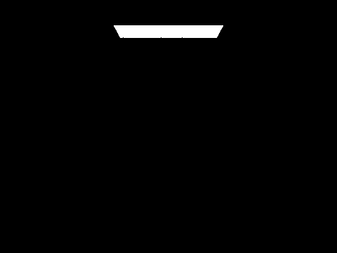
|

|

|

|

|
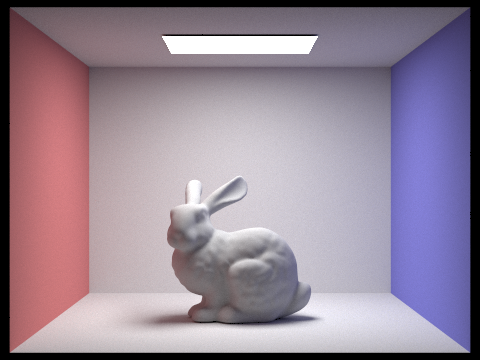
|

|

|
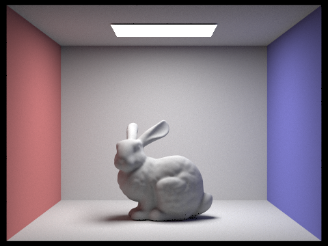
|

|

|

|

|

|

|

|

|

|

|
As you can see, I have burned up my computer rending all of this at 2am.
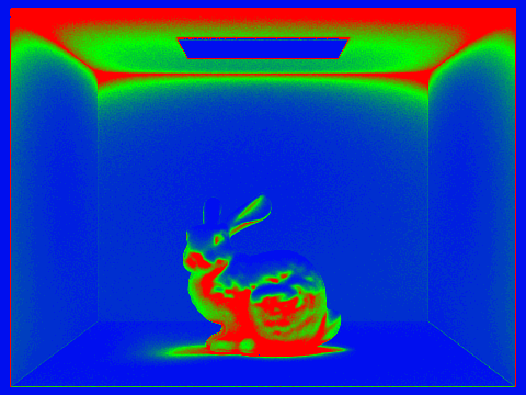
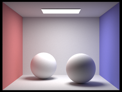
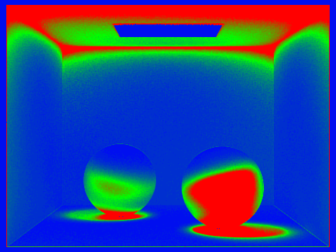
The idea for adaptive sampling is that normally, we choose a num_samples amount of times to sample each pixel. After sampling each pixel a lot, we usually get a pretty good idea of what it will look like. However, this takes too much time and a lot of times, we don't need to sample the pixel nearly that much to get an accurate representation of it. So with adaptive sampling, we still sample each pixel multiple times, but we also check all the samples taken for that pixel ever so often. We then perform a z-test by converting the data taken into standard normal form and compare see if the confidence interval is sufficiently small. In this case, we are using the 95% confidence interval, so we stop when we are 95% sure that the actual average pixel color is within our interval. Since we are now pretty sure that our pixel is good enough and that additional samples won't do much to change the color, we are done with this pixel and can move onto the next pixel. My implementation of this process involves keeping track of the s1 and s2 values at all times, as well as n, the current number of samples taken. Then, for every batch size samples, aka when n mod (batch size) = 0, we compute the mean, sd, and I of the current samples taken by using s1, s2 and n. If I is less than or equal to maxTolerance times the mean, then we exit. We also exit when n reaches the actual max num samples per batch. I then update the rate with the value of n.

|
|
|
|