Overview
Overall, this homework was very interesting and we've learned a lot about the rasterization process and ways to reduce aliasing. I thought barycentric coordinates were a very cool concept and an ingenious way to smoothly interpolate values inside triangles. Perhaps the most interesting thing we've learned from the homework is how well we are able to make images that are pretty much just as good as supersampling without actually supersampling. Supersampling is an intuitive solution to aliasing, but it uses astronomically large amounts of space and time, and with some combination of bilinear pixel sampling and linear or nearest level sampling, we can basically replicate that effect with less overall complexity. It really goes to show how people have thought of clever solutions to reduce aliasing and properly rasterize objects and textures.
Section I: Rasterization
Part 1: Rasterizing single-color triangles
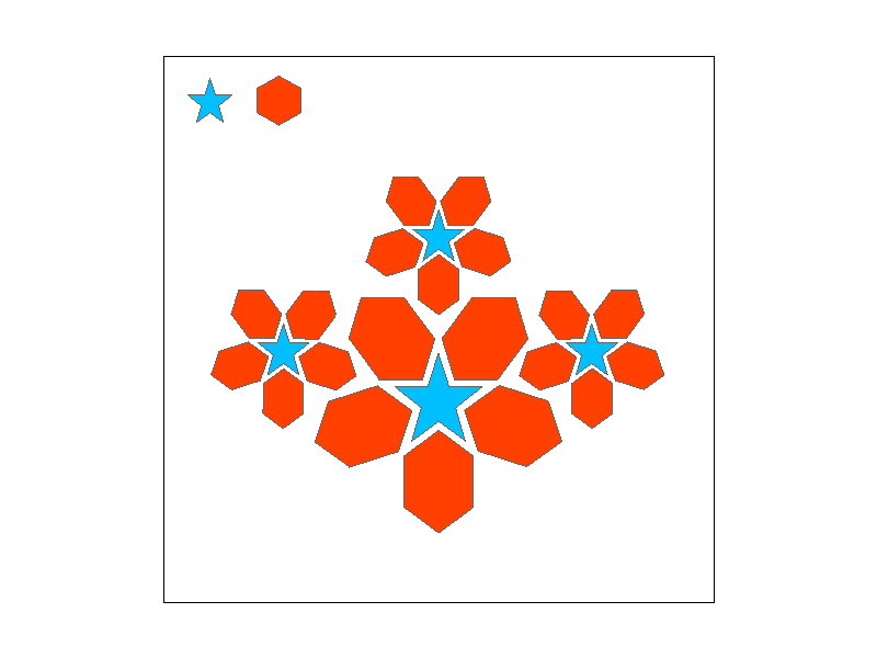
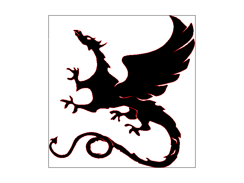
In task one, we implemented basic triangle raterization in a very lecture/textbook like way. For each triangle, we sample the points in a rectangle around the triangle, going from the lowest X and Y values of the given points from the triangle and sampling column by column until we reach the very highest X and Y values of the given points. We can achieve this by using floor(min()) of all the X and Y points for the starting point, and ceil(max()) of the X and Y values for the given points for the finishing value. Then, once we have the starting and finishing points, to make future calculations easier, we first calculate the value of all dXi = Xi+1 - Xi, and the same for the Y values of all points. In other words, we first generate the line tangent vectors needed for determining whether a point is within a triangle or not. After this, we have the X and Y values for the 3 line vectors, so we enter a loop, iterating from our predetermined start point and going column by column (no reason in particular we choose to iteratre through Y values first rather than row by row) until we reach the finishing value. Then, since the current X and Y values we have are ints and we want to sample from the middle of each pixel, 0.5 is added to the X and Y values before it is used in the calculations. Now, with the proper values we want to sample, we use the formula Li(x,y) = -(x - Xi)dYi + (y-Yi)dXi to see if any given point is within a given line, running this equation for all lines. Since we didn't account for orientation, we know that a point is within the triangle if all three line tests are positive or negative. So after L0, L1, and L2 have been generated by the equation, we check if all of them are either positive or negative, and if that's the case, then we fill the pixel with the original coordinates x and y (before 0.5 was added) with the given color.
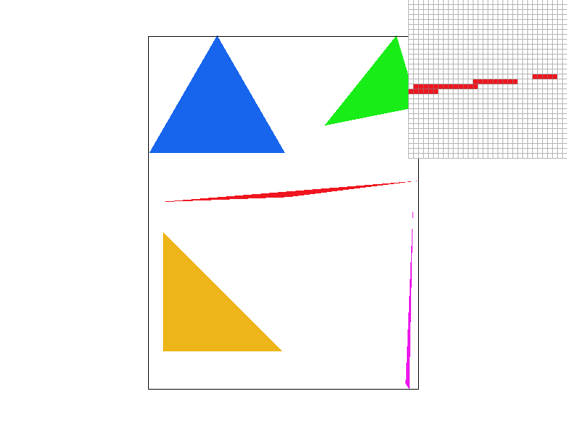
After implementing task 2, we now have two additional for loops in the rasterize_triangle function to account for the additional subpixel samples needed for each sample. When supersampling is turned off however, the function acts the same as when supersampling hasn't been implemented, and samples from each X and Y pixel value in the bounding box plus 0.5, or the middle of each pixel. Our algorithm is no worse than an algorithm that checks every pixel within the bounding box for each triangle because that's exactly what it does: check each pixel in the bounding box for each triangle.
|
|
|
|
|
Part 2: Antialiasing triangles
To implement supersampling, we added two additional for loops to the rasterize_triangle function for subpixel sampling. These for loops sample root(sample_rate) extra times in both the X and Y axis, for a total of sample_rate additional samples. To do this, we first calculate rate=sqrt(sample_rate), and then we set each for loop to loop rate times. The for loops iterates an xn and yn variable, which keeps track of which current supersample is being carried out. For each subpixel sample, we take the original X and Y value for the sample, which points at the upper left of the pixel, and set the sample as x + (1/rate) * (xn + 0.5) and vice versa for y. This equation first splits the pixel into 1/xn * rate boxes, and in each box we sample in the middle, which is why we add 0.5. This allows the subpixel samples to be evenly distributed around the pixel. To account for the extra samples, we changed sample_buffer's size (dynamically) based on the sampling rate, and "downsampled" when writing to the frame buffer, averaging the colors of all the samples within each pixel. To do this, we made sure that whenever the sample buffer was resized, its size was multiplied by sample_rate to account for the sample_rate extra samples for each pixel. When writing from the sample buffer to the frame buffer, we had to average out the values of sample_rate samples to write to each sample in the frame buffer. We did this with a double for loop similar to the one used in rasterize_triangle, adding all the color of all the samples together and dividing them by the sample_rate. Finally, we write the color to the frame buffer as usual.
In addition, we had to change fill_pixel to accommodate for supersampling in a similar way that we changed resolve_to_framebuffer, but instead of averaging out several pixels to fit one pixel, we make it so that it fills several pixels rather than one pixel. In essence, pixels are now sampled several times when rasterizing triangles, and the sample buffer is exanded to fix this change. The old fill_pixel function doesn't accomodate for this change and only fills in pixels in their original positions, not in their supersampled positions. So we made it so that fill_pixel fills in the correct pixel as well as the surrounding pixels that would have been results of supersampling at that pixel location with the same color. Since fill_pixel is use by rasterize_line and rasterize_point, by making this change, we fix the border that is drawn in during around the rasterized image during most of the tests.
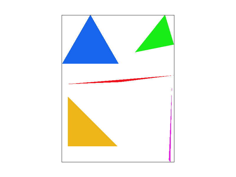
Supersampling is useful because it averages out colors on the edges of shapes, giving a smoother look and combatting aliasing. Without supersampling, edges of shapes look very jagged. By implementing supersampling, we were able to make the edges of our triangles look much smoother as the pixels on the edges of triangles were averaged instead of one color or the other.
|
|

|
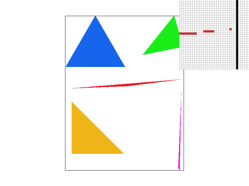
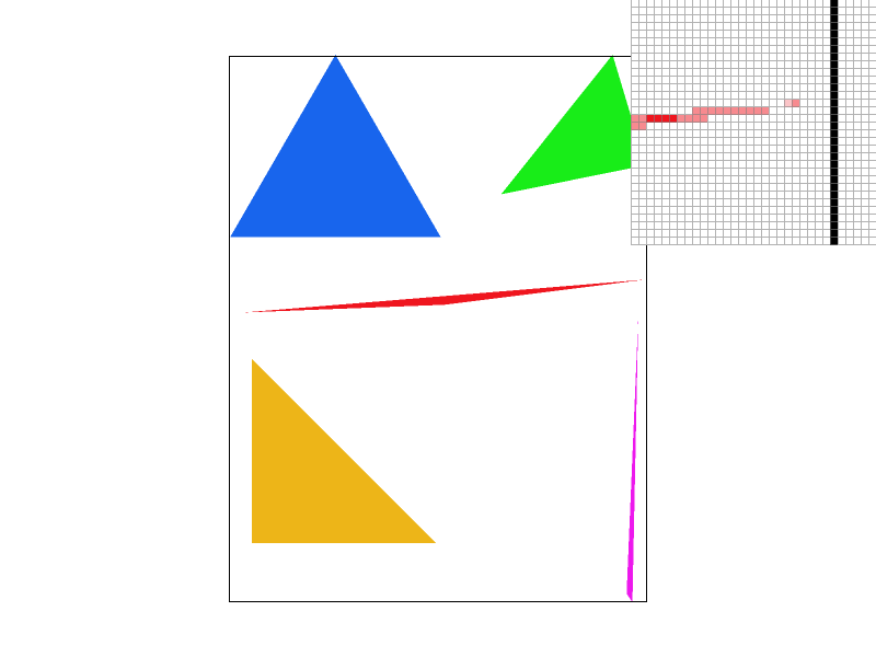
When the sample rate is 1, there is no supersampling, so there are artifacts of sampling present (the pixels detached from the triangle). When we raise the sampling rate to 4 we see a bit more smooth of an edge on the triangle. Some of the pixels are clearly averaged from red and white. When we raise the sampling rate to 16 we see a much smoother edge. This is because the higher the sampling rate, the more accurate the average is at estimating the portion of the pixel that is on the inside of the triangle.
Part 3: Transforms
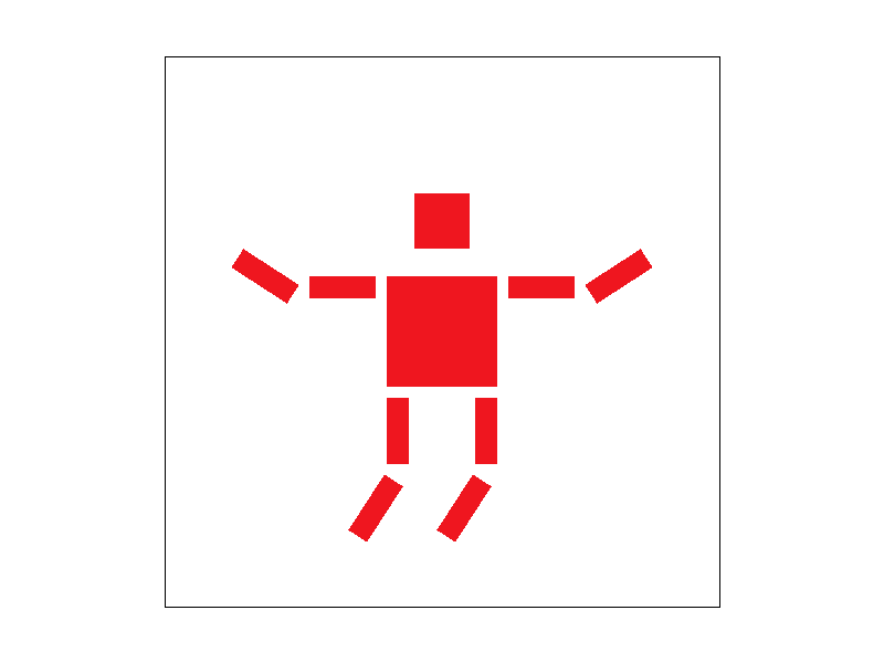
|
We were trying to make him look like he is jumping with his arms out, so we rotated and translated the bottom parts of his legs, and the outer parts of his arms.
For transforms, we have to provide a 3x3 matrix for the that will transform the position vector appropriately when multiplied together. To do this, since matrices are just row major arrays, we created a 9 length array of doubles for each transform with the identity matrix as a base. Then, for translation, we added the x and y values to translate by to the M02 and M12 spots of the identity matrix, respectively, and returned this matrix. For scale, we replaced the M00 and M11 values, which are previously 1 from the identity matrix, to the given sx and sy values to scale by. For rotate, we had cos(deg) and -sin(deg) in spots M00 and M01, and sin(deg) and cos(deg) in spots M10 and M11.
Section II: Sampling
Part 4: Barycentric coordinates
Barycentric coordinates are three numbers, alpha, beta, and gamma, which add up to 1. The coordinates are each assigned to a corner basically describe how much the point is being "pulled" towards each corner. For example, if alpha=1 and beta and gamma are 0, then the point is exactly at the alpha corner. If the coordinates are all about equal, the the point is likely somewhere near the middle of the triangle.
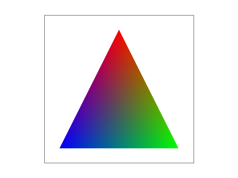
To demonstrate our implementation, here we have a triangle that smoothly interpolates between red, green, and blue. Notice how the Notice how the color is a smooth gradient that becomes more blue as it approaches the left corner, more red as it approaches the top corner, and more green as it approaches the right corner. This represents the barycentric coordinates for each respective corner, where as a point approaches a certain corner, its respective coordinate (alpha, beta or gamma) becomes larger and the other coordintes become smaller, so the color becomes more solid with less influence from other colors. When looking near the middle of the triangle, the color appears to look gray-ish, which represents how each corner has an equal influence on the final color.
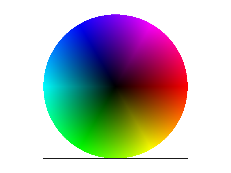
Pixel sampling is the process in which we apply textures to shapes. So we have some object with a mesh that is made up of lots of triangles. To display a certain pattern or color on this mesh, we use textures, which are basically patterns that we can slap onto objects and give it color. However, objects can be any size shape or form, and may be a different size or shape than the original texture. To map the textures onto the object successfully, we need to use pixel sampling, which takes the object's spacial and texture coordinates and samples the correct colors from the given texture. One way to do this is with nearest pixel sampling. First, to determine the right texture coordinates, we find the barycentric coordinates using the current spatial coordinates we are sampling at and multiply that by the texture coordinates at each point. Then, we take these texture coordinates and simply round it to the nearest whole number to find the closest real texture pixels to the coordinates and return that. For bilinear sampling, we instead look at the 4 nearest texels to that texture sampling point, and use linear interpolation to weight the final color based on the colors of the 4 nearest texels, weighted by how far they are from the sampling location. We then return this color.
Part 5: "Pixel sampling" for texture mapping
|
|

|

|
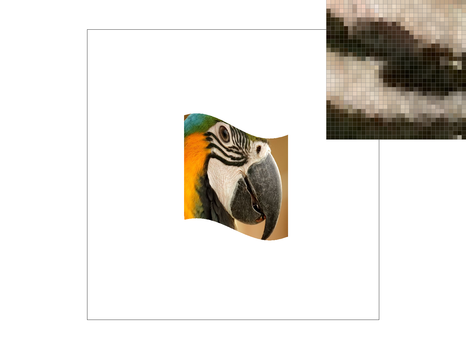
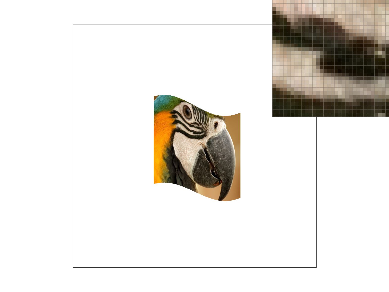
With nearest pixel sampling and no supersampling, the edges of the pattern are sharp and jagged. With bilinear sampling, the edges are noticably smoother. However, with supersampling, both bilinear and nearest sampling look similar and are both pretty smooth. This is because supersampling does essentially the same thing as bilinear sampling, except it averages out the colors after they have been pulled from the texture, and bilinear sampling takes into account the nearest texels while sampling. Either way, a large difference between nearest and bilinear sampling will only been seen with no or little supersampling.
Part 6: "Level sampling" with mipmaps for texture mapping
We now move onto level sampling. Previous, when sampling texels, we always pulled them from mipmap level 0, which is basically the full texture. However, there are times when we want to sample from a lower resolution version of the texture, namely when we are zooming out a lot, in which case there will be aliasing if we are using the full resolution texture. However, this low resolution image will appear blury and low resolution when zoomed in. So with level sampling, we can dynamically alter the resolution/mipmap level of the texture when texture sampling based on the magnification of the object to reduce aliasing. To do this, when we take the sample and convert it to texture coordinates, we also take the sample location 1 pixel to the right and a sample 1 pixel up and convert those to textrue coordinates. Using these new texture coordinates, we compare those to the original sampling location and determine whichever one is the most furthest away, and we take the log2 of this value to use as our mipmap level. Breaking this process down, we first take the max difference in texture sampling location between the original location and the location to the up and right. We do this because this lets us get an idea of how "stretched" the texture is: if the next coordinate is very close, then the texture is likely very magnified (since 1 unit in real space barely amounted to any change in texture space, so a lot of real space is used to hold the texture, so the texture is very magnified.). In this case, we want to use a lower mipmap level which provides a higher resolution image, and we use log2 of the value since each mipmap level is bigger/smaller that the last by a power of 2. If the next sample location is very far away on the texture, then the texture is very minimized, as it means that we have the entire texture covering very little real space, so the texture is probably very far away from the camera. In this case, we want to use a lower resolution image of the texture or a higher mipmap level, so log2 of the value will also provide us the proper mipmap level.
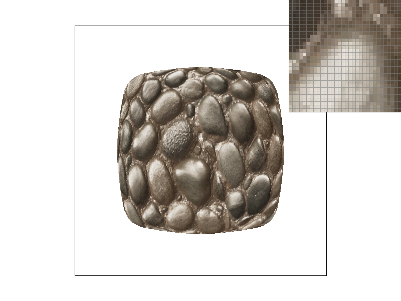
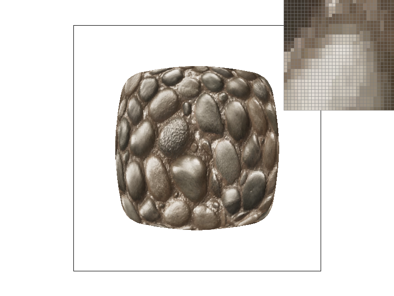
Now, we have a few extra level sampling techniques. Originally we were just always using mipmap level 0, but now we can also choose to use nearest or linear level sampling methods. Basically what this means is that after we use the previously described technique to find log2(max difference of texture sample locations), we now have some decimal. With nearest level sampling, we simply round this to the nearest whole number and use that number as the mipmap level for pixel sampling. With linear level sampling, we take take this number, L, and pixel sample on the nearest whole numbers to L for mipmap levels. We then take the results of these samples and weight them by L itself, as in if L is 0.5, then we weight the samples equally, and if L is closer to one whole number than the other, then we weight the sample that used that mipmap level more. Performance wise, always using mipmap level 0 along with using nearest pixel sampling would be the fastest, but would result in lots of aliasing. This is perhaps permissable if you use supersampling at a high rate, but supersampling is very computationally intensive and it seems as though people want to avoid it at all costs. Supersampling also uses a lot more memory as it requires the sample buffer to be much larger, which is another thing that people probably want to avoid. Moving on, using bilinear pixel sampling results in a much smoother and almost supersample-like image with not as much performance cost as supersampling. By using nearest level sampling, we can achieve a slightly better picture at a bit more of a performance cost. Using linear level sampling requires a lot more computational power, but results in a much smoother image especially when combined with bilinear pixel sampling. This is trilinear sampling, and is basically only second to supersampling in terms of smoothness but still uses less memory and performance. At the end of the day, the best image and optimal amount of smoothness is subjective, though it has a formula behind it. Persomally I don't like when the image is far too smooth, as I think it looses some amount of detail.
|

|
|

|
