|
|
|
We first implement a virtual camera so that we can generate camera rays into the scene. Then, we implemented ray intersections with objects or primitives in the scene. However, simply generating rays into the scene and checking if they intersect and finally rendering can take some time so we implmented Bounding Volume Hierarchy. This is done in order to decrease the amount of interesection tests taken which in turn decreases the render times. Next, we implemented direct illumination to simulate light and how its rays would behave after interacting with an object. With direct illumination, we only care about light rays hitting an object which subsequently reflects those rays into the camera. This is a fundamental step in implementing indirect illumination where we simulate light rays bouncing multiple times with multiple objects before finally reaching our camera. After implementing how light rays behave, we implemented adaptive sampling which reduces the amount of samples we use per pixel depending on how much samples the individual pixel needs to get rid of noise. While going through our samples for the pixel, every couple of samples we check their mean and standard deviation to see if the samples are already close enough a similar that we can stop sampling but still have a non-noisy scene. This allows us for quicker rendering as we can reduce the samples of pixels that don't need as much as the maximum_samples count.
First, we have to implement camera rays. To do this, we have to map the given normalized image (x, y) points to camera space by using linear interpolation. After the given points are in camera space, or on the virtual sensor plane, we can create a ray in camera space by making a direction vector start at the camera's origin and stopping at the transformed coordinates. This ray is then transformed to a ray in world space and then normalized. Now, we can sample a pixel for our framebuffer.
We sample a pixel for our framebuffer by randomly generating rays for the desired pixel and averaging the rays' radiance. For this, we have to use `est_radiance_global_illumination` function to estimate the radiance along a ray that we specify.
Now that we can sample pixels. We can implement ray intersecting with objects, triangles and spheres. We can check for intersection for triangles by setting the ray equation equal to the plane containing the triangle; similarly, for spheres, we can set the ray equation to the sphere equation. For both, we solve for t which if between `min_t` and `max_t` will mean that there is an intersection. `min_t` and `max_t` represents the minimum and maximum distance traveled along the ray from the ray's origin.
For ray-triangle intersection, since the triangle is in a plane, we have to check if the ray intersects with the plane as well but also make sure it intersects inside the triangle and not outside of it. This could be done by finding the barycentric coordinates of the point of intersection; to do this, we used Moller Trumbore algorithm to efficiently find the barycentric coordinates and to find t. Once t is found, we have to check if it is within `min_t` and `max_t` and that the barycentric coordinates are within 0 and 1.
With ray-sphere intersection, a ray can intersect two times (ray passes through sphere twice), once (ray is tangent to a point on sphere), or none (ray doesn't touch the sphere at all) at all. This is what solving for t tells us. For the case with intersecting two times, we will take the intersection point that happens first or is closer to the ray. Then, as mentioned above, we check if it is within the ray's `min_t` and `max_t`.
|
|
|
|
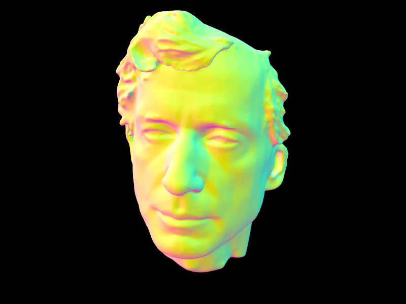
Bounding Volume Hierarchy for the mesh is implemented because it significantly improves render time. By organizing objects or primitives into a hierarchical tree, we reduce the number of intersection tests required leading to faster render times. BVH essentially reduces the need to test for intersection for improves render time.
When constructing our BVH, we use a recursive approach where we first compute the bounding box of a list of primitives and initialize a new BVHNode with that bounding box. If there are no more than `max_leaf_size` primitives in the list, we know it is a leaf node so we just have to update its start and end iterators and end the recursion.
Otherwise, we divide the primitives into a left and right collection. To do this, we have to find the split point to split the bounding box of primitives. We determine the splitting point by first choosing an axis containing the most information; this would be the axis with the most spread out primitives. We can easily find this by using the current recursion call's bounding box's extent and choosing the biggest extent axis. Then, we can find the average centroid along this axis. This would be our splitting point.
We now use the splitting point, the average centroid, to seperate the primitives to a "left" and "right" collection. We simply do this by creating two vectors, one for left and the other for right collection, and then put the primitives smaller than or equal to the average centroid in the left vector. Similarly, we put the primitives larger than average centroid in the right vector. Then, we need to reassign the pointers so that the primitives in the left vector come first before the ones in the right vector. Then, we recurse for the BVHNode's left and right nodes.
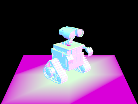
With BVH: Average speed 3.5431 million rays per second. With BVH: Averaged 5.791015 intersection tests per ray. |
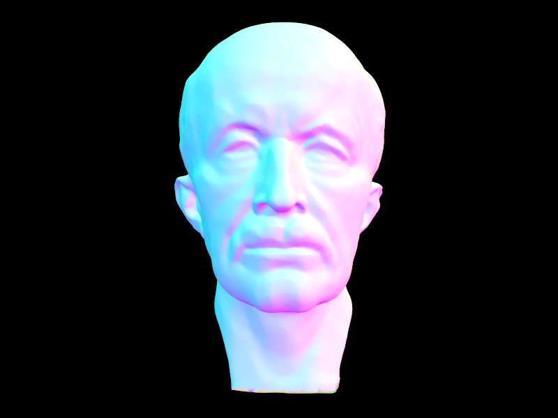
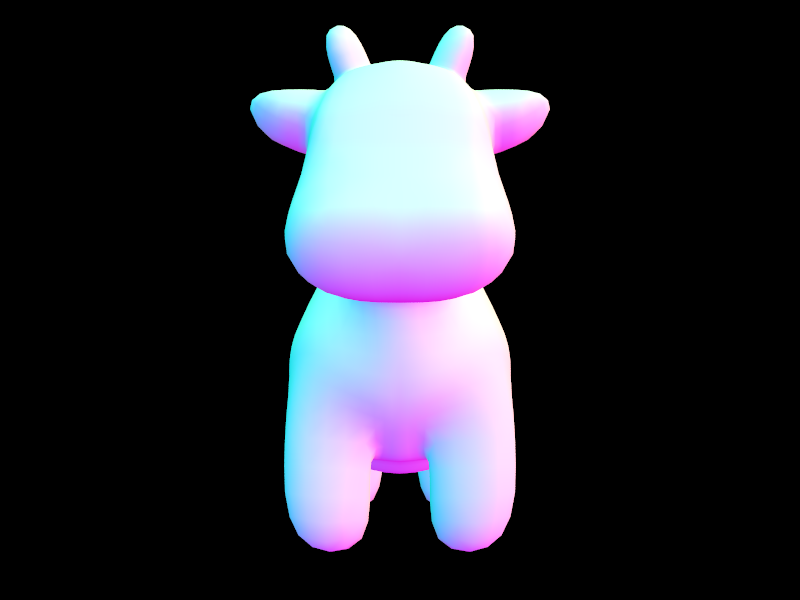
With BVH: Average speed 3.9021 million rays per second. With BVH: Averaged 5.188529 intersection tests per ray. |
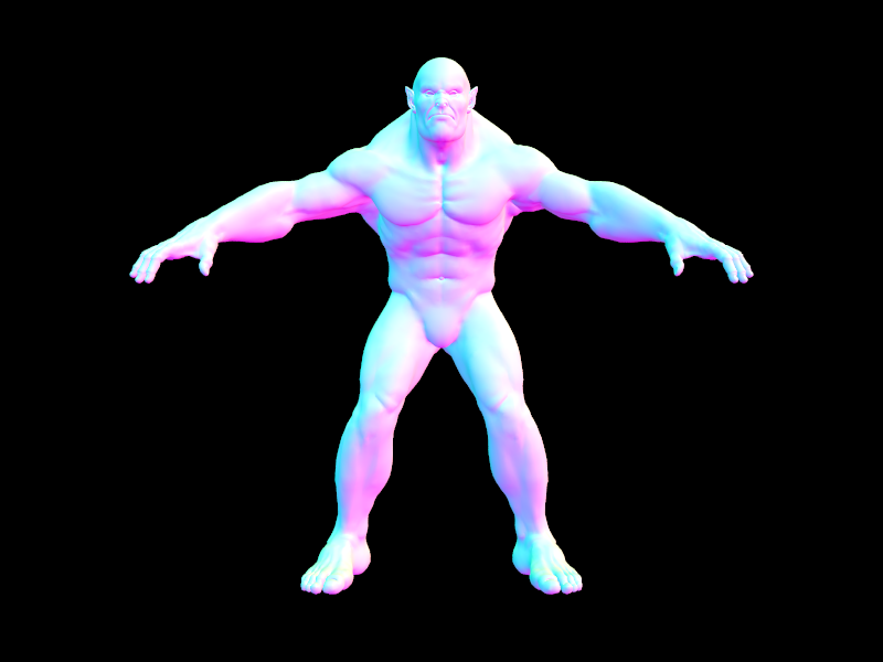
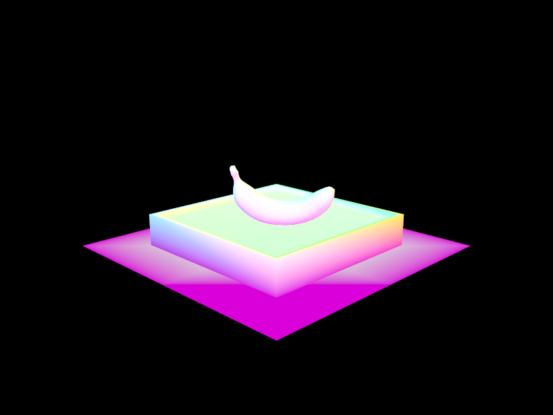
With BVH: Average speed 3.1452 million rays per second. With BVH: Averaged 3.702847 intersection tests per ray. |
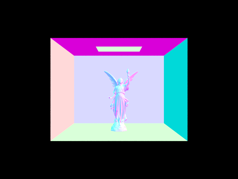
With BVH: Average speed 3.0944 million rays per second. With BVH: Averaged 4.455590 intersection tests per ray. |
|
With BVH: Average speed 3.1452 million rays per second. With BVH: Averaged 3.702847 intersection tests per ray. Without BVH: Average speed 0.0012 million rays per second. Without BVH: Averaged 47566.375856 intersection tests per ray. |
With BVH: Average speed 6.0633 million rays per second. With BVH: Averaged 5.320804 intersection tests per ray. Without BVH: Average speed 0.0748 million rays per second. Without BVH: Averaged 1408.421536 intersection tests per ray. |
With BVH: Average speed 5.5163 million rays per second.
With BVH: Averaged 2.551915 intersection tests per ray.
Without BVH: Average speed 0.1930 million rays per second.
Without BVH: Averaged 592.024120 intersection tests per ray.
CBlucy takes the longest to render, then the cow, and finally the banana without BVH. Generally, without BVH, the time to render a scene will increase as the complexity of the scene increases. Therefore, BVH is necessary since it reduces render times significantly. Looking at the number of intersection tests per ray, we can see that our BVH is working. BVH skips intersection tests that are unnecessary and instead only check relevant primitives for intersection. For example, without BVH, CBlucy averaged about 48,000 intersection tests whereas with BVH, it averaged only about 4 -- a significant improvement. Similar results for cow.dae and banana.dae.
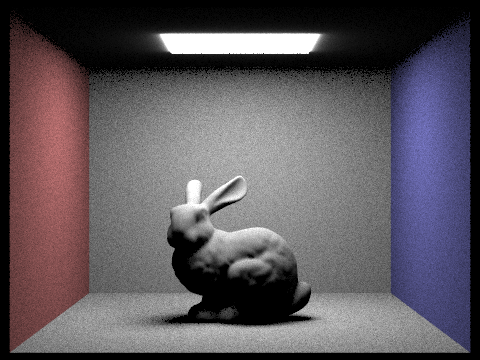
Direct illumination is implemented by tracing inverse rays (instead of rays from light source to camera, we trace rays from camera to light source) to determine if a point is lit by a light source in the scene. Essentially, we trace rays outward from the intersection point, check for intersections with any light sources, and color the pixel depending on the irradiance at the intersection point. We implmented direct lighting or illumination two ways: uniform hemisphere sampling and importance sampling.
For implementing uniform hemisphere sampling, we approximate the irradiance at the given intersection point by sampling direction vectors from the hemisphere. Then, we create rays that are defined by the intersection point and the the sampled direction. These rays would essentially be the rays reflected by the object. We would then use these rays and test for intersection with other objects in the scene. In the case of estimating direct lighting by uniform hemisphere, we only care about these rays intersecting a light source. We sum the radiance emitted (which is calculated by multiplying the BSDF and the angle of the sampled direction). After this, we estimate the outgoing radiance, `L_out`, by dividing by the number of hemisphere directions sampled, `num_samples` as well as the pdf which is the probability of each sampled direction.
For implementing importance sampling, we instead sample direction vectors from the light source from the given intersection point. We do this by making normalized direction vectors between the hit point and the light source. Similar to what we did with uniform hemisphere sampling, we do intersection tests but only for points between the the intersection point and the light source. For rays with no intersection, we sum the radiance emitted (calculated by weighting BSDF, cos theta, and pdf). This gives us the Monte Carlo estimate for outgoing radiance at the point for a specific light source. For all light sources, we simply add the outgoing radiances to get the total outgoing radiance of the point.
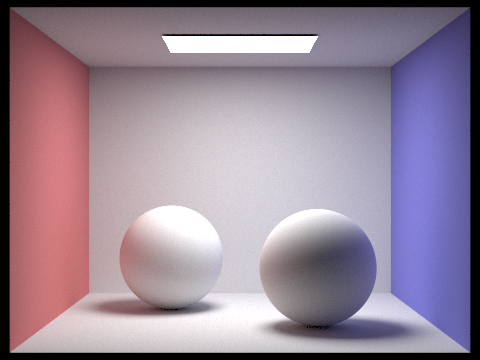
| Uniform Hemisphere Sampling | Light Sampling |
|---|---|
|

|
|
|

|

|
|

|
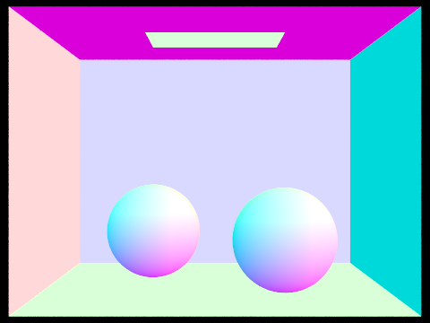
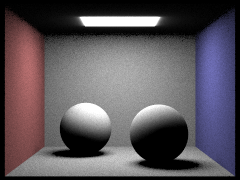
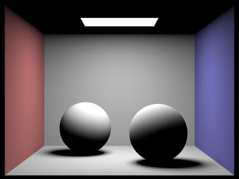
The more incoming light rays that we take into account to calculate outgoing light, the more accurate our image’s lighting is. As you can see, while the the scene rendered with only 1 light ray is very noisy, the scene rendered with 64 light rays is a lot more clear. This is because, with direct illumination, we are counting on taking an estimate and average to calculate the outgoing rays. The more samples we can use in calculating the estimate, the more accurate our estimate can be.
Overall, the uniform hemisphere sampling results are much noisier than the lighting sampling results, however, it also has more texture than the lighting sampling results. Because of uniform hemisphere’s randomness in finding samples, its understandable that the scene can be more noisy than lighting sampling that looks at the individual light objects in the scene. However, the random sampling also allows the uniform hemisphere sampling to be closer to a global illumination in the sense that it takes in a different ray each time. This allows the scene to have a more textured and natural look while lighting sampling looks glossy.
For implementing the indirect lighting function, we start out by adding one_bounce_radiance to Lout, the returning sum of radiance. We then essentially keep tracing ray bouncings for max_ray_depth amount of rays, until our russian roulette stops it, or if there is no more intersection for the next ray.
|
|
|
|
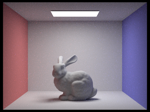
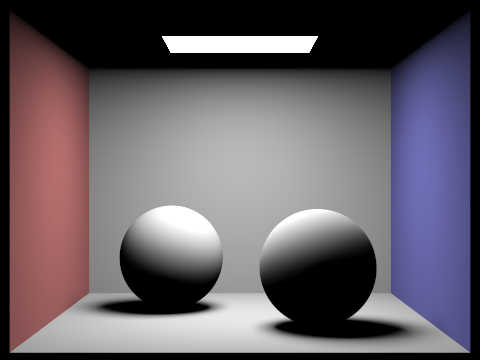
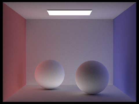
Although both scenes are visible and rendered with some light showing the scene, the only direct illumination seems brighter, but the only indirect illumination seems more complete and realistic. This makes sense because the only direct illumination uses only the first bounce of lighting, which is the most brightest because it has diffused the least amount of times. However, there is more of a contrast between the light and dark regions because all pixels are either lit or not, there is no spectrum for it. In contrast, the only indirect illumination looks more natural and fluid in the lighting because it takes in an accumulation of all the different indirect lighting hitting the pixel.
|

|

|

|

|
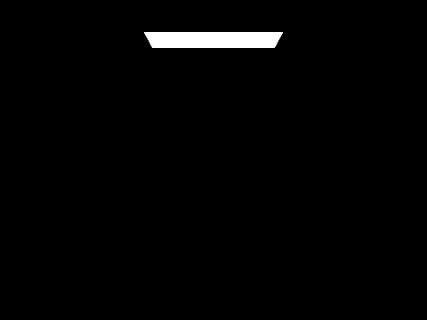
The max_ray_depth 0 and 1 are working as expected. With a max_ray_depth of 0, it is basically saying only take in zero_bounce_radiance. With a max_ray_depth of 1, it is basically rendering a one_bounce_radiance scene. Both of these scenes we have seen before and know it is working as expected. As for max_ray_depths of 2, 3, and 100, it is a sharp contrast of max_ray_depth of 0 and 1, and they are a lot more similar to each other. For these max_ray_depths, it is also implementing at_least_one_bounce_radiance. Any max_ray_depths greater than 2 still uses at_least_one_bounce_radiance, but makes the lighting slightly more accurate each time.
|
|
|
|
|
|
|
|
|
|
|
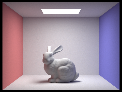
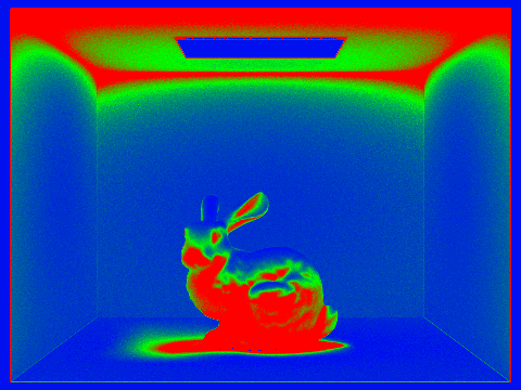
The rendered views are working as expected, as the scene is getting less noisy as the sample-per-pixel rate increases. This makes sense because with more samples to work with per pixel, the accuracy of lighting is more set and controlled. Because we are sampling uniformly random, low sample rates can be dangerous because the randomly chosen sample could be wrong. However, with many random samples, it guarantees a fairly accurate result.
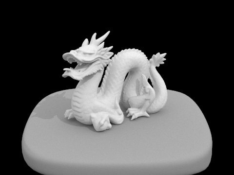
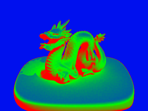
Adaptive sampling is a method used to efficiently render scenes by only sampling as much as the pixel needs requires to get rid of noise, which is different for different pixels. Because of global illumination, some pixels’ illumination are much more complex and are made up of more indirect lighting than others. This various complexity means that each pixel requires a different amount of sampling to get a non-noisy result, therefore the amount of sampling per pixel is adaptive. We implemented this adaptive sampling method by checking the precision of the sample values in the pixel. While iterating through the max number of samples per pixel, every samplesPerBatch number of samples, we check the precision of the samples. Using the formulas in the homework spec, we find the mean and standard deviation of the samples and check if their deviation is within a MaxTolerance. If the samples are within the tolerance range, it means the samples are close enough that we can stop sampling because it should not be noisy anymore. If the samples never reach this MaxTolerance, then the pixel would just be sampled the maximum amount of times. However, this method allows the code to quit the loop sooner than the maximum amount of times if allowed.
|
|
|
|