CS 184: Computer Graphics, Spring 2024

Project 2: MeshEdit

Henry Khaung, Aaron Xu

Overview

Implemented Bezier curves and expanded them to also work on 3D surfaces. Then, implemented Phong shading so that meshes can have better shading. Finally, implemented loop subdivision to increase resolution for low resolution polygon meshes by implementing local remesh operations `flipEdge` and `splitEdge`.


Task 1: Bezier Curves with 1D de Casteljau Subdivision

In this task, we implemented de Casteljau's algorithm for 1D which is useful for finding Bezier curves.

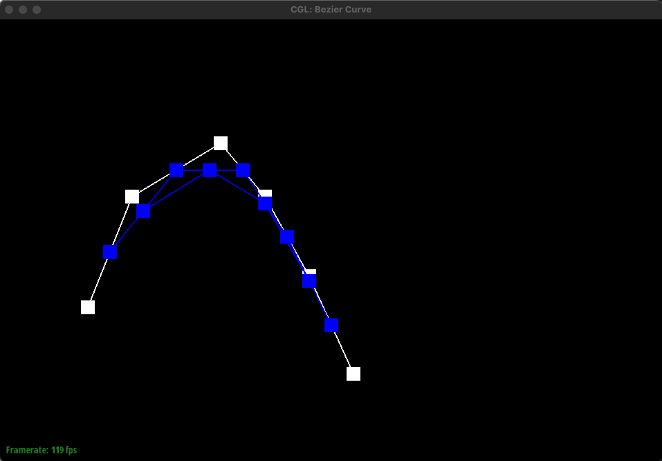
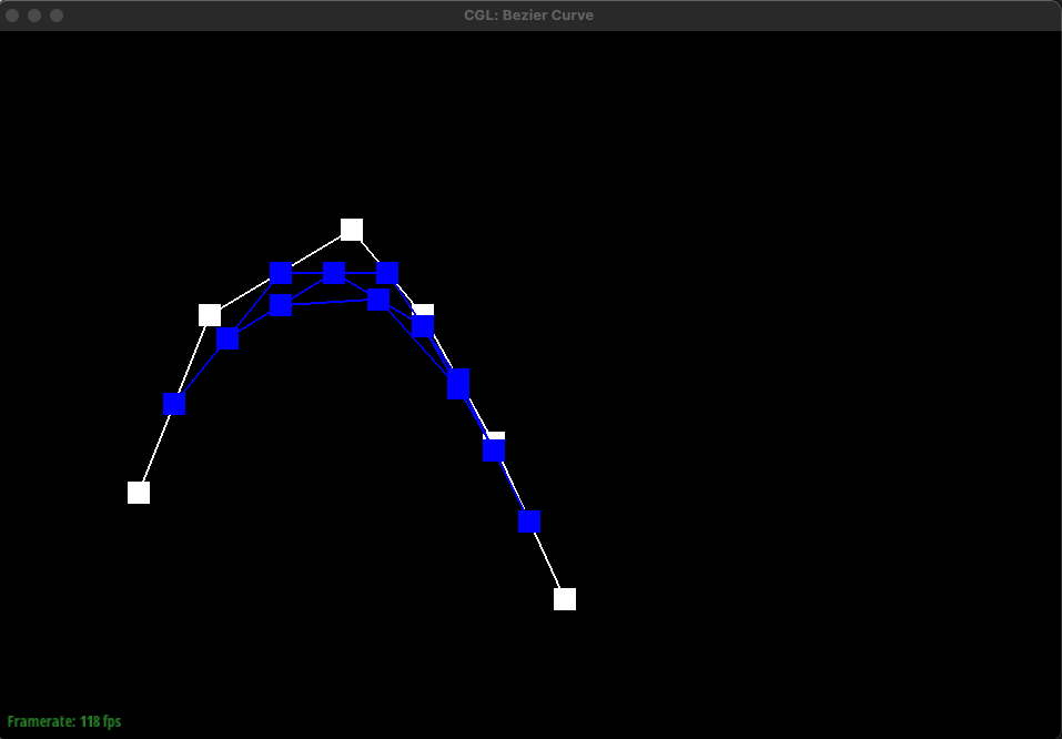
de Casteljau's algorithm takes the given control points, inserts a point using linear interpolation between each control point, and does this recursively until we are left with only one point. Essentially, it recursively finds intermediate control points between each pair of given control points using linear interpolation until only one point remains. This enables for a smooth curve.

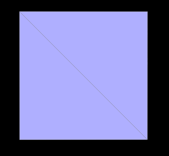
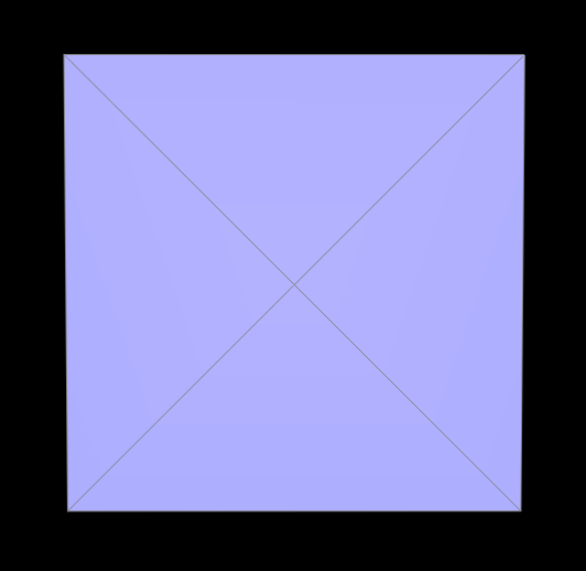
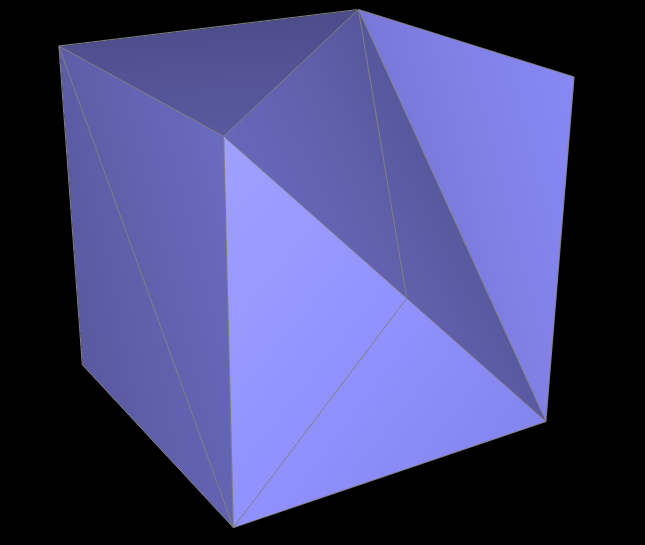
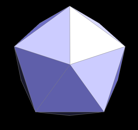
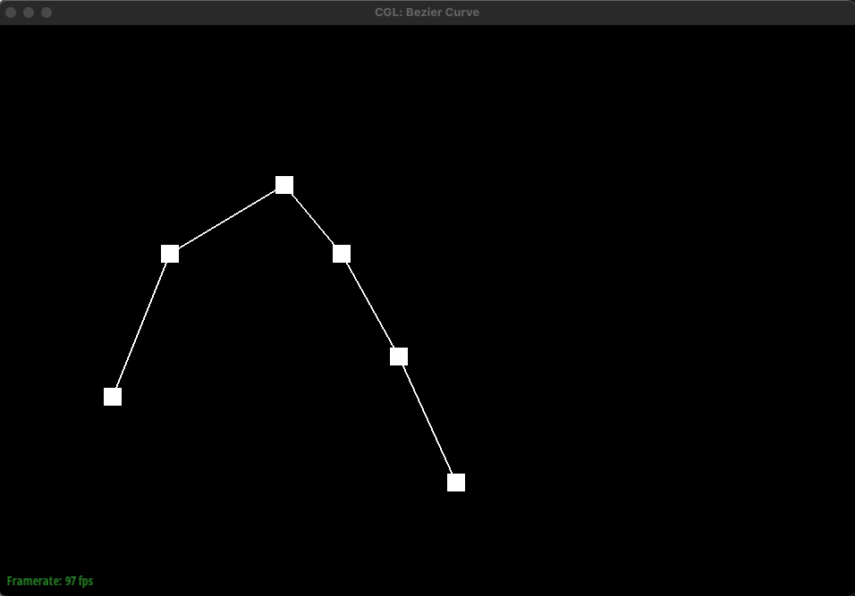
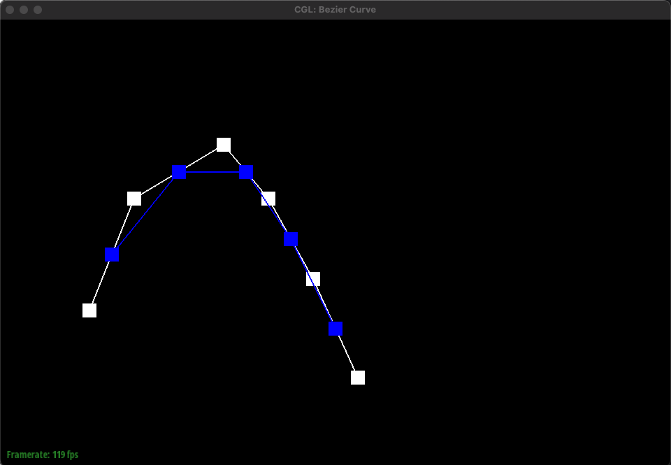
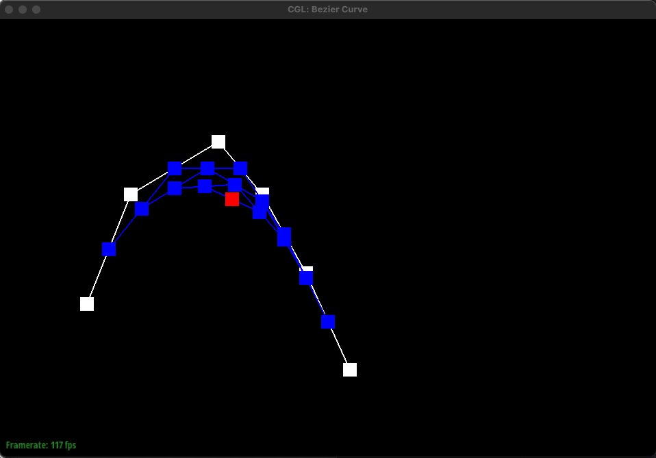
The implementation is straightforward. Simply iterate through the given control points, which is a list of points (x, y) and during the iteration, perform linear interpolation between the current point and the next point and add this interpolated point to a new list of points. This new list containing intermediate points is returned. Eventually, this new list will only contain one final point that lies on the Bezier curve. This final point is the red point shown below in the images.


Given 6 control points
evaluateStep is called once
evaluateStep is called twice
evaluateStep is called three times
evaluateStep is called four times
Final intermediate point with completed bezier curve!

when parameter t is changed

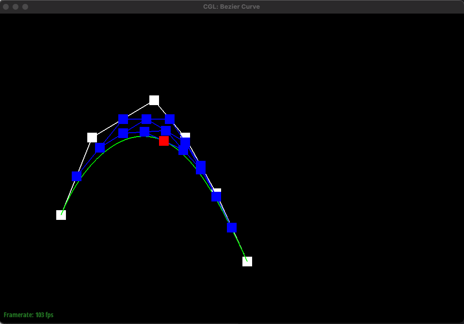
If we have 6 control points, we would have to do linear interpolation 5 times to get 5 intermediate control points for the first step of de Casteljau's algorithm. Then, with these 5 points, we would have to do linear interpolation 4 times to get 4 intermediate points. This repeats until we have one final control point as shown above in the images. Essentially, given n points, we have to find n-1 intermediate points using linear interpolation until we are left with one final point that lies on the Bezier curve. This algorithm is used to find the bezier curve as indicated by the green curve above.

The parameter t ranges from 0 to 1 and determines the position of the final intermediate point. For example, when t = 0, this corresponds to the starting point. In the gif above, it would be the leftmost and bottommost point whereas when t = 1, this corresponds to the last point which is the rightmost and bottommost point. The parameter t essentially controls how far along the curve the interpolated point should be.


Task 2: Bezier Surfaces with Separable 1D de Casteljau

In this task, we extended de Casteljau's algorithm to work with surfaces.

Instead of working with a list of 2D coordinates, we are now given a grid, or matrix, of 3D coordinates. We first find Bezier curve points for each row of points using de Casteljau's algorithm. Then, we find the Bezier surface point on the computed Bezier curve points.

  • `evaluateStep`

    This function is called when we want to evaluate the next step of de Casteljau's algorithm and is a helper function for `evaluate1D`. It is the same logic as the `evaluateStep` function for BezierCurve except we work with 3D coordinates.

  • `evaluate1D`

    This function is called when we want to fully evaluate de Casteljau's algorithm given a list of control points and pararmeter t. It calls `evaluateStep` until we are left with one final point which would be the evaluated curve point.

  • `evaluate`

    This function finds us the Bezier surface point given a grid of control points and parameters u and v by making use of the helper functions from above: `evaluate1D` and `evaluateStep`. As mentioned above, we first perform de Casteljau's algorithm on the rows using parameter u to find Bezier curve points. Then, the final surface point is determined by again calling `evaluate1D` but instead with parameter v.

Screenshot of bez/teapot.bez


Task 3: Area-Weighted Vertex Normals

In this task, we implemented area-weighted normal vectors at vertices. These vertex normals can be used for Phong shading which is a better shading for smooth shading compared to flat shading.

To implement this, we find all the neighboring faces that share the given vertex and for each face, find the area and normal. Then, compute the area weighted norm. We can then sum all the area weighted norms of each face and normalize it. This would be the unit normal at the given vertex.


Teapot without shading (without vertex normals)
Teapot with shading

Task 4: Edge Flip

In this task, we implemented a remeshing operation on an edge. This operation flips an edge by changing its two endpoints, or vertices, to another pair of vertices.

To implement this, we wrote down a list of all elements: half-edges, vertices, edges, and faces in a simple mesh. The simple mesh consists of two triangles glued together by a half-edge. This list of elements represents what the elements were originally pointing to before the flip operation. This list is important because it ensures that we do not forget to reassign the pointers after the flip operation. Finally, we perform the flip operation by changing the given edge's two vertices to the other two vertices in the simple mesh and reassigning all pointers. Keeping track of all elements and doing so correctly was crucial in ensuring that they were no bugs in this function. This required a complete understanding of the halfedge data structure which we did not have initially. We were confused with halfedge->vertex; we initially thought halfedge->vertex meant the vertex pointed to by the halfedge. After fully understanding how the halfedge datastructure worked, we were able to easily implement the flip operation.


Teapot before any flip operation
Teapot after some flip operations

Task 5: Edge Split

In this task, we implemented a remeshing operation on an edge. This operation splits the given edge and inserts a new vertex at the midpoint and connects the two opposing vertex that were not originally connected by the given edge.

Implementing this was similar to the implementation of `flipEdge` except now, we have to account for new elements. To implement this, we first drew a diagram of two triangles connected by a half-edge before the split. We labeled every pointer in the diagram before we perform the operation just like we did in `flipEdge`: halfedges, vertices, edges, and faces. In code, we tracked all these pointers. Then, we drew a diagram of what would happen to these two triangles after the split operation and labeled what each pointer would point to. In code, this is done by using `setNeighbor` function; we also had to create new halfedges, new vertices, new edges, and faces which is done by calling `newHalfedge`, `newVertex`, `newEdge`, and `newFace`. Overall, these diagrams were key in helping us implement this function because they helped us easily determine what each pointer should be reassigned to.


Before any edge splits
After an edge split
After some edge splits and edge flips

Task 6: Loop Subdivision for Mesh Upsampling

In this task, we implement loop subdivision which increases the number of triangles in the mesh. This way, we can convert a low resolution polygon mesh into a higher resolution. This is a similar concept to supersampling in antialiasing.

To implement this,

  1. We computed new positions for all the vertices in the input mesh and stored these new positions in the `newPosition` property of the `Vertex` class. To compute a new position, we can use the following formula:
    (1 - n * u) * original_position + u * original_neighbor_position_sum
    where n is the degree of the current vertex, u is a constant dependent on n, original_position is the original position of the current vertex, and original_neighbor_position_sum is the sum of all neighboring vertices' positions. When n is 3, then u is 3/16; otherwise, u is 3/(8 * n).

  2. Then, we computed the new vertex positions and stored it in `newPosition` property of the `Edge` class. The new vertex positions are calculated using the following formula:
    3/8 * (A + B) + 1/8 * (C + D)
    where A and B are the positions of the vertices that share the edge that connects two triangles together and C and D are the positions of the other vertices of each of the two triangles.

  3. Then, we split every edge in the mesh that is old, or in the original mesh, using the `splitEdge` function. This returns a midpoint vertex which we set its position to the new position we stored in `newPosition` of the `Edge` class.

  4. After this, we flip any new edge that connects an old and new vertex.

  5. We then set the new vertex positions for every vertex.

Following these steps, we were able to make the upsample function work. However, it did not produce the expected results. There were two bugs. Initially, the upsample function creates a mesh with all the faces missing. This was because we did not set any edges to be `isNew` after splitting. After this was fixed, we encountered an error where the upsampled mesh results in a mesh that is missing polygons. This was not a bug from the upsample function but rather a bug from our `splitEdge` function. The problem was fixed by properly reassigning all the pointers, new and old, of the input mesh of the function.

After loop subdivision, sharp corners and edges become smoother since the number of polygons in the mesh are increased. You can reduce this effect by pre-splitting edges near the sharp corners and edges.


Before subdivision

After subdivision, it becomes rounded

After pre-splitting edges around sharp corners and subdivision

Viewing the mesh from the side shows us that the sharp corner is somewhat maintained

Similarly, the cube is not symmetrical after repeated subdivisions because originally, for each of its faces, it only has one inner edge which causes it to be asymmetric. The fix is to pre-split this edge for each face and then do subdivision.


This inner edge highlighted white makes the cube asymmetrical. The fix is to pre-split!

Asymmetric after repeated subdivisions

Splitting the white edge once and doing this for all faces will make the cube symmetrical.

The cube is now symmetric!