In this assignment, we implemented rendering of Bezier curves and surfaces in addition to rendering of triangles meshes. Bezier curves (and subsequently surfaces) are built using the de Casteljau algorithm and Phong shading was applied to render Bezier surfaces. Unlike the previous rasterizer assignment, this assignment requires the use of half-edge data structures which define triangle meshes. We implement flipping and splitting on edges in halfedge-defined meshes, then use these features to upscale the meshes using loop subdivision. As extra credit we also designed our own model in Blender and supported loop subdivision for boundary edges. An additional feature we implemented was a screenshot hotkey (as in homework 1) with minimal text blurring and a black background (instead of transparency).
Given a set of $n$ control points and timestep $0 \leq t \geq$, de Casteljau's algorithm finds $n-1$ intermediate points between each consecutive pair. When this step is applied recursively until one point remains, we eventually find the single point on the bezier curve at $t$.
In part 1, we implemented one step of de Casteljau in evaluateStep. For each pair of control points $p_i$ and $p_{i + 1}$, we compute the intermediate point $q_i$ by using linear interpolation.
$$q_i = lerp(p_i, p_{i+1}, t) = (1-t) p_i + t p_{i+1}$$To store the result of this calculation we push results into a C++ stdlib vector of Vector2D objects. The last point at index $n-1$ ($n$ being the size of the input points vector) is excluded since de Casteljau requires a subsequent control point.
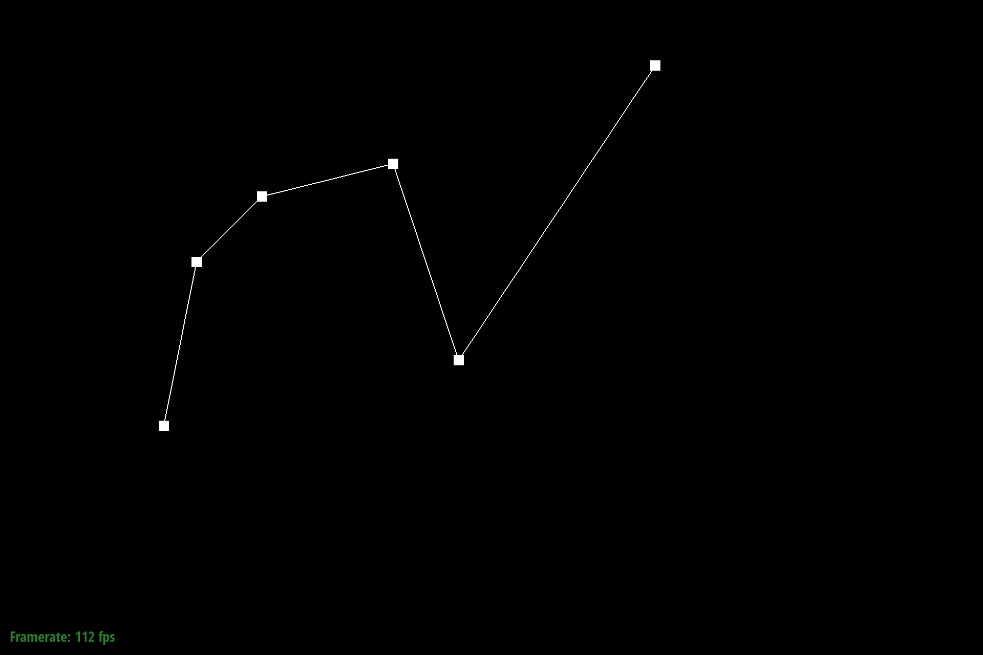 Figure 1: Bezier control points at L0 |
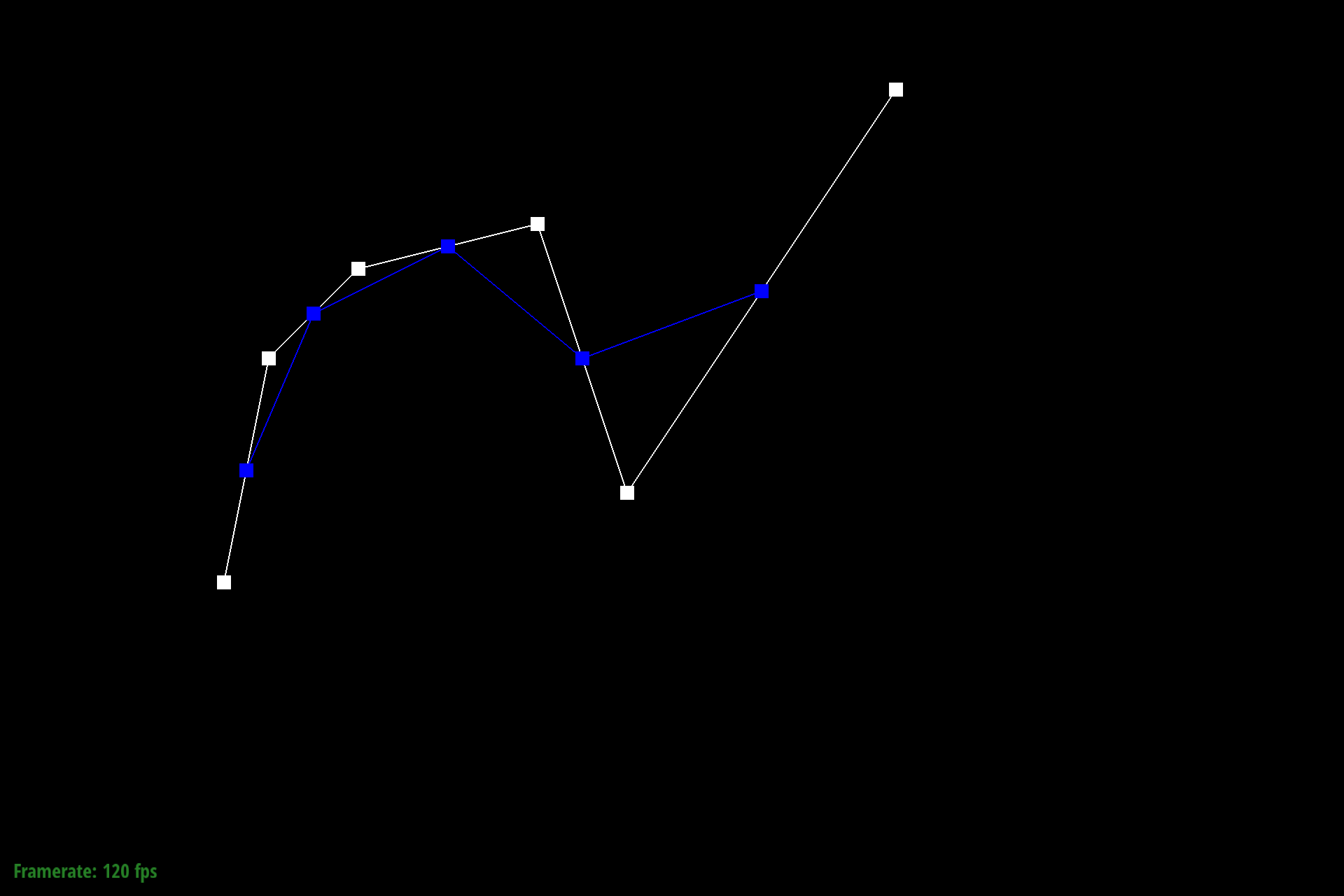 Figure 2: Bezier control points at L1 |
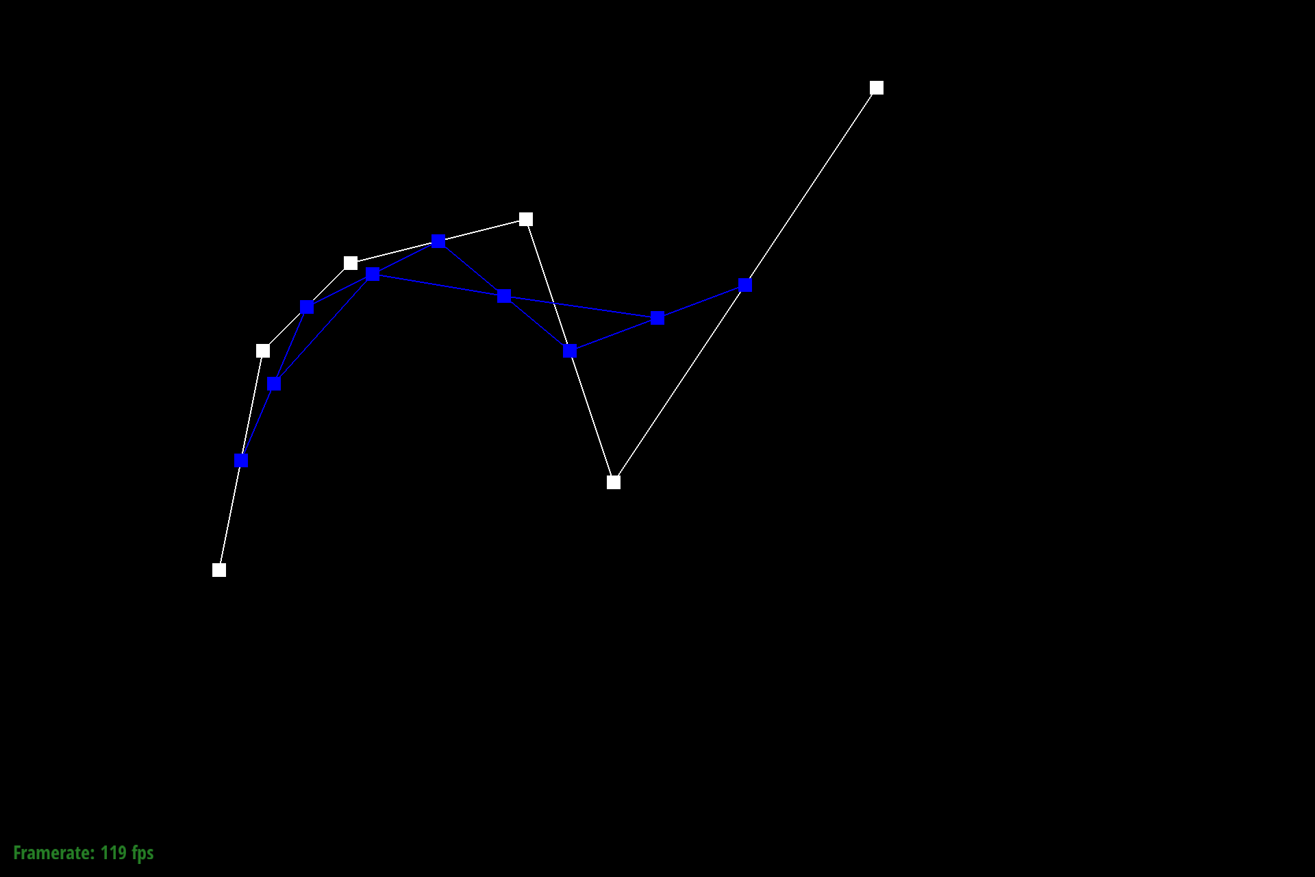 Figure 3: Bezier control points at L2 |
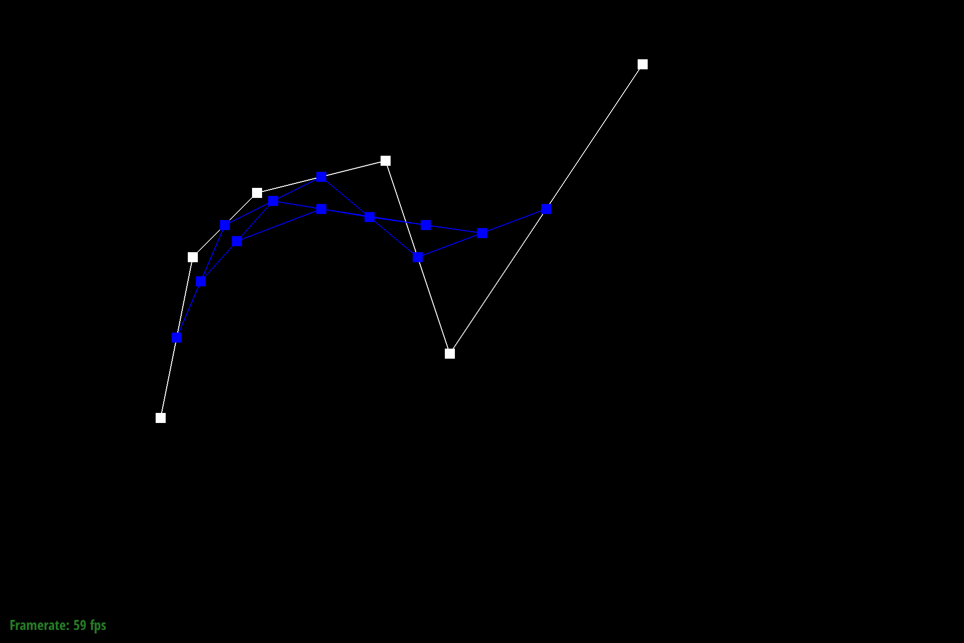 Figure 4: Bezier control points at L3 |
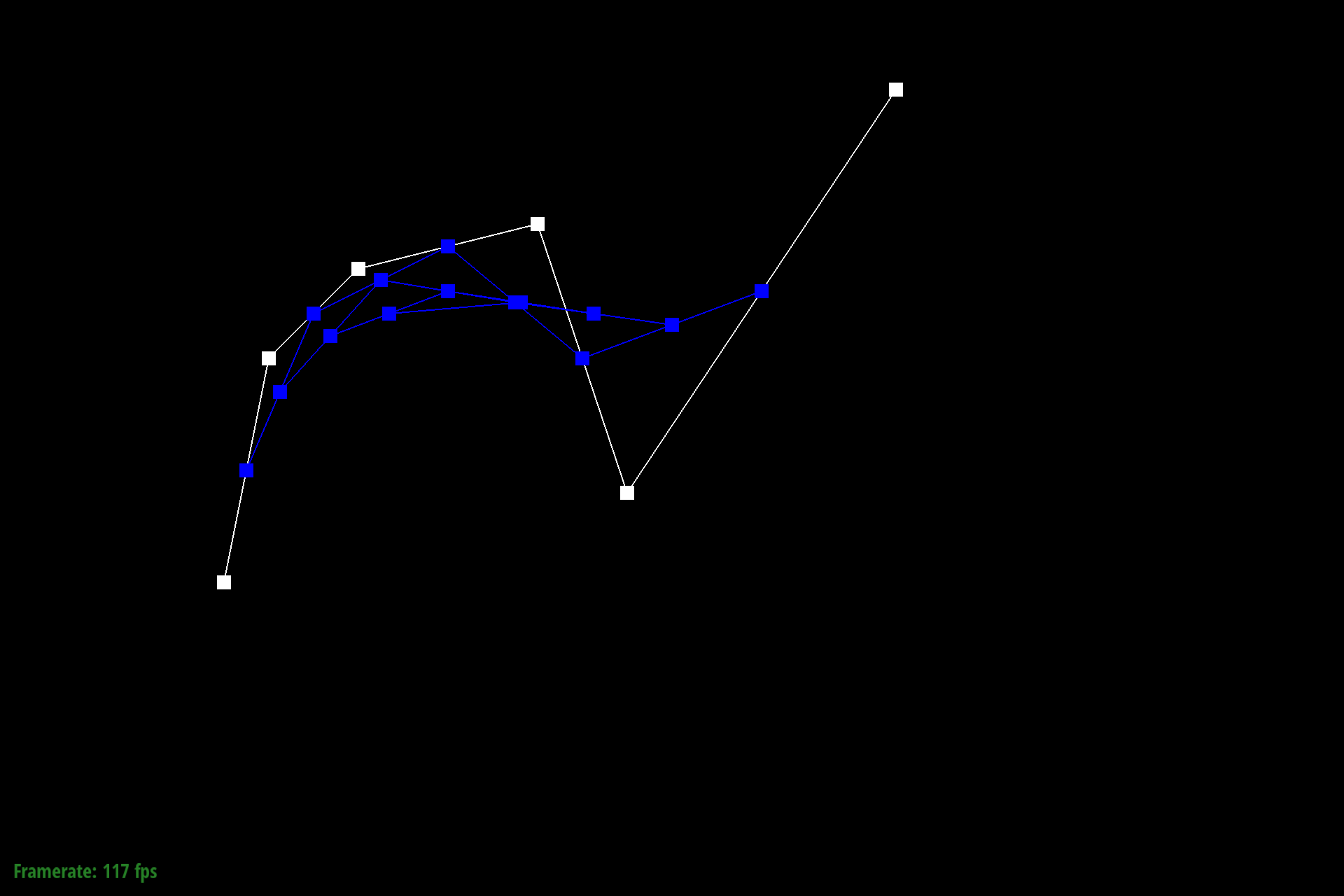 Figure 5: Bezier control points at L4 |
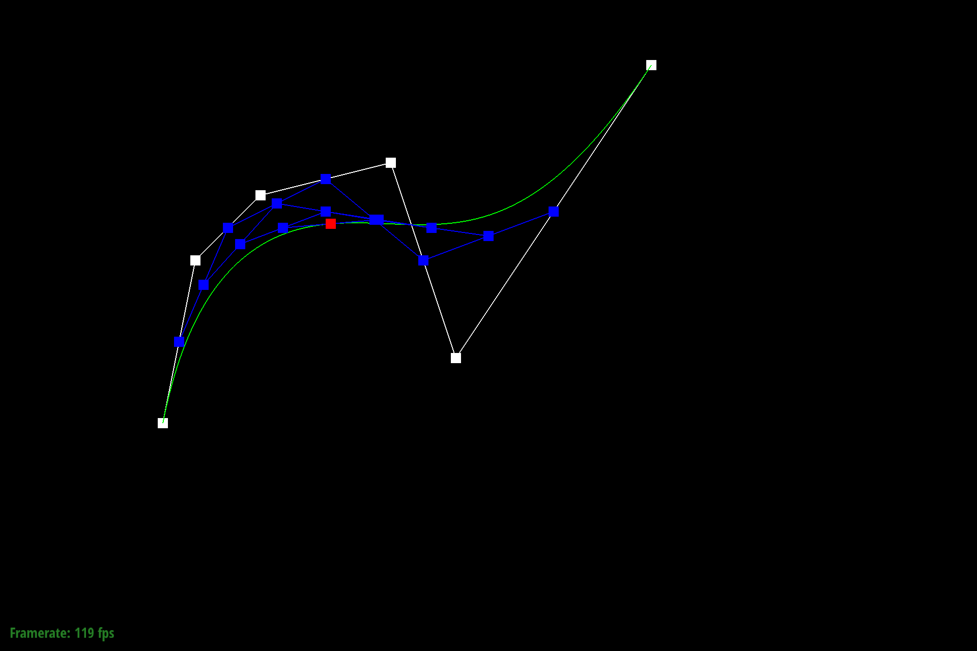 Figure 6: Bezier control points at L5 |
The below images show a different Bezier curve with a varying $t$.
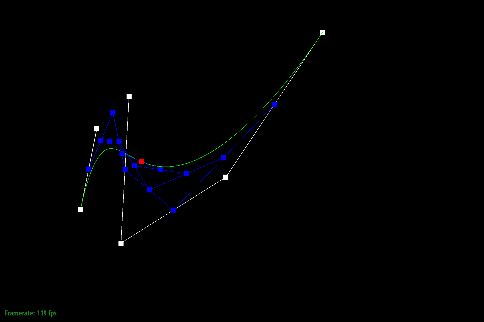 Figure 7: Different Bezier curve at nominal $t$ |
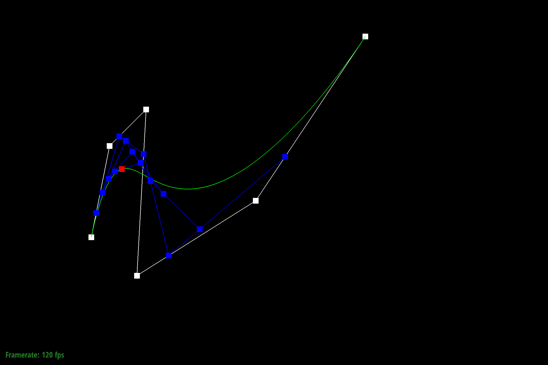 Figure 8: Different Bezier curve at decreased $t$ |
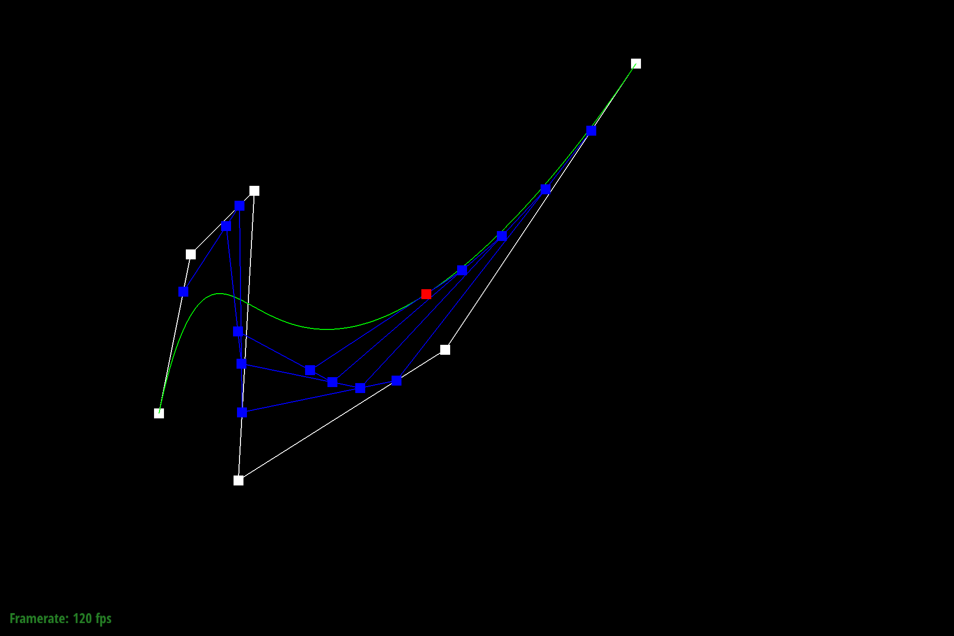 Figure 9: Different Bezier curve at increased $t$ |
To implement Bezier surfaces, we take in an $n \times n$ matrix of control points $P_{ij}$ and two parameters $u$ and $v$; we apply a similar process for Bezier curves with a few key additions.
For each row of $n$ control points $P_{i0},...,P_{i(n-1)}$, we evaluate it at parameter $u$, resulting in $n$ control points for the "moving" Bezier curve. Once each row has been processed, we use these control points to evaluate $v$ on the "moving" curve. Essentially, to extend de Casteljau's algorithm from Bezier curves to Bezier surfaces, we generate multiple curves and interpolate between each consecutive pair to create another curve in the third dimension which generates the point on the Bezier surface at $(u, v)$. This algorithm is carried out by the function BezierPatch::evaluate(...) with the helper methods BezierPatch::evaluate1D(...) and BezierPatch::evaluateStep(...).
- BezierPatch::evaluateStep(...): Given a set of control points and timestep $t$, return the intermediate points. This function is the same as the one used in part 1 for Bezier curves except std::vector<Vector3D> is returned rather than std::vector<Vector2D>.
- BezierPatch::evaluate1D(...): Fully evaluate de Casteljau's algorithm by calling BezierPatch::evaluateStep(...) recursively until one point remains. This final interpolated point is then returned.
- BezierPatch::evaluate(...): Given an $n \times n$ matrix of control points and $(u, v)$, we call evaluate1D(...) on each row at $u$ to generate a Bezier curve in the $u$ direction. Afterward, points on these curves are evaluated in the $v$ direction.
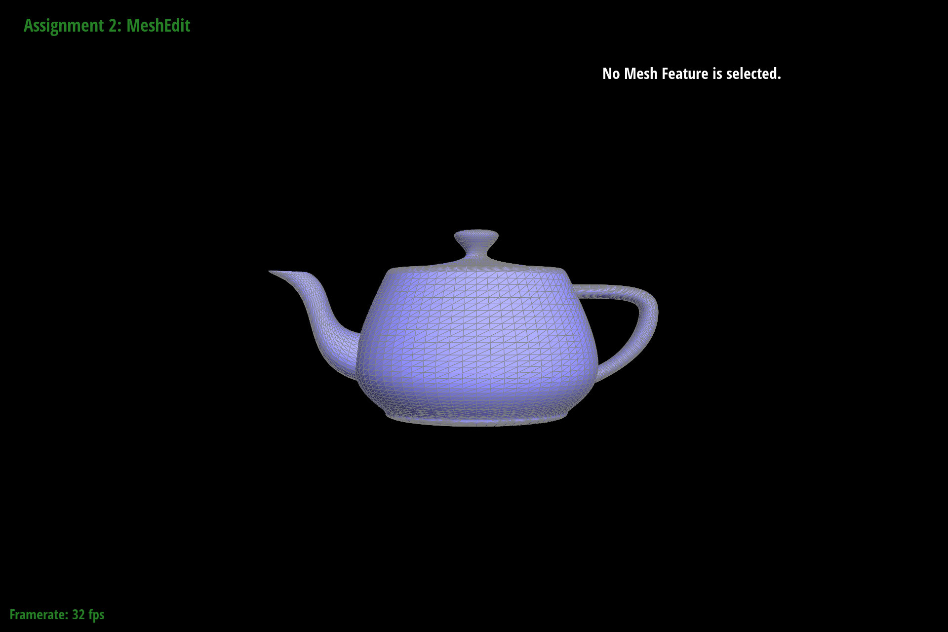
Figure 10: teapot.bez evaluated by the de Casteljau algorithm
To implement area-weighted normal vectors at vertices, we weight the normal of each face by its area and take the average.
We first start at the halfedge of the current vertex $h$. To find the vertices of the adjacent halfedges, we use the functions next() and vertex() in the Vertex class. We then use the vertex positions to compute the cross product of the two edges of the triangle which outputs the area-weighted normal vector of the current triangle. This value is then added to our running sum vector result. To traverse to the next face, we assign $h$ to be the next outgoing half-edge of the vertex h = h->twin()->next(); . After iterating through all incident faces until we return to the original half edge, we take the sum of all area-weighted normal vectors and normalize it so that it has unit norm.
As a result of implementing Phong shading, the shading becomes smoother for smooth surfaces compared to flat shading.
 Figure 11: teapot.dae with flat shading |
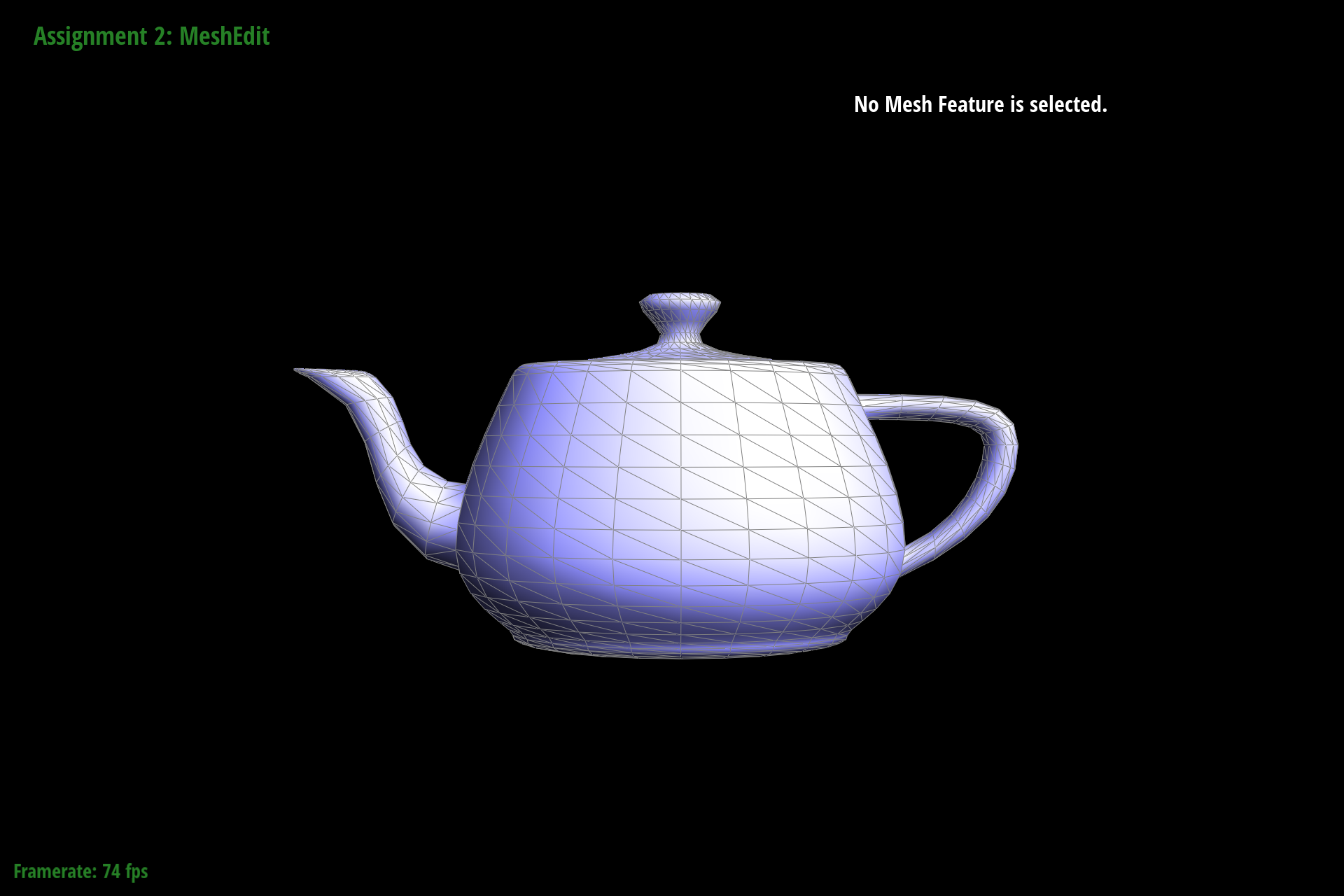 Figure 12: teapot.dae with Phong shading |
In this task, we implement an edge flip operation. This is accomplished through manipulating the pointers stored by the selected edge object.
To begin, we started by drawing out a hypothetical mesh with two triangles. Drawing from the halfedge data structure, each edge has two halfedges; one on each side. Each point in the mesh is a vertex, and every enclosed space is a face. In the example, this would make for a total of 5 edges, 10 halfedges, 4 vertices, and 2 faces.
A hand drawing of this is included below. Note that we choose to use the convention of having twin edges labeled as $h_{Xt}$. So for example the halfedge $h_0$ has a twin $h_{0t}$. The t stands for "twin" and is a way to denote inner and outer edges. The inner edges are $h_X$ while the outer are $h_{Xt}$. Also, see that the halfedge corresponding to the original edge is $h_0$, and each next halfedge increments this number. When we reach the end of the first triangle, ordering is applied to keep the edge count increasing on the outside of the mesh i.e. $e_0$ then $e_1$ then $e_2$ etc.
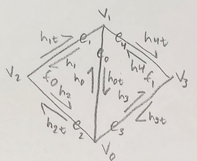 Figure 13: Triangle mesh with labeled components |
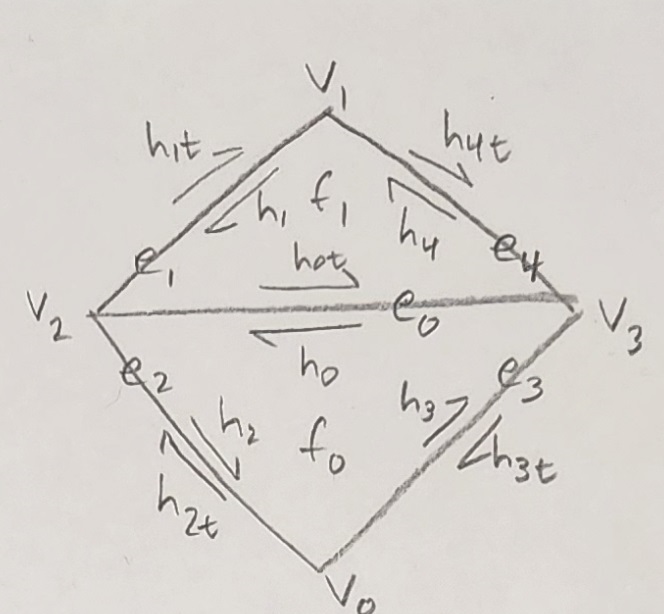 Figure 14: Triangle mesh with labeled components after edge flip |
The flip operation does not create or destroy any of these mesh components. Instead, it reallocates their properties (in pointer form) to move the single inner edge to the other two vertices. Primarily, this means the inner edges all have a new set of neighbors corresponding to the diagram above. Secondarily, the faces and vertices are assigned new halfedges. A vertex's halfedge is one which begins from that vertex. If there are multiple halfedges originating at a single vertex, one is chosen arbitrarily. Similarly, a face's halfedge is any halfedge in that face, chosen arbitrarily. None of the outer halfedges need to be modified as they are all still connected to the same external mesh components.
To check if an edge is a boundary, we simply check isBoundary() on the selected edge. If true, we return the original edge $e_0$ immediately. If not, we continue to the rest of the function described above. The normal return value is then a destructively modified $e_0$.
In debugging, we primarily relied on viewing the mesh in the GUI and selecting different components. By noting the address and comparing it to other objects, we could see where pointers were being assigned and if they were being assigned correctly. As a trick to make debugging faster, we truncated addresses to the last 4 digits since most components around a mesh seemed to be unique in that address space. Originally we tried with 3, but that led to some components being mistaken for each other that were in fact distinct in the fourth digit. We also ended up using temporary variables to store all halfedges, twinned halfedges, faces, edges, and vertices following my naming format outlined above. This saved debugging time by making it significantly easier to spot neighbor assignment issues just from looking at variable names.
The images below show an example teapot.dae model with (1) no edge flips, (2) one diagonal edge flip, and (3) one diagonal edge flip and one horizontal edge flip
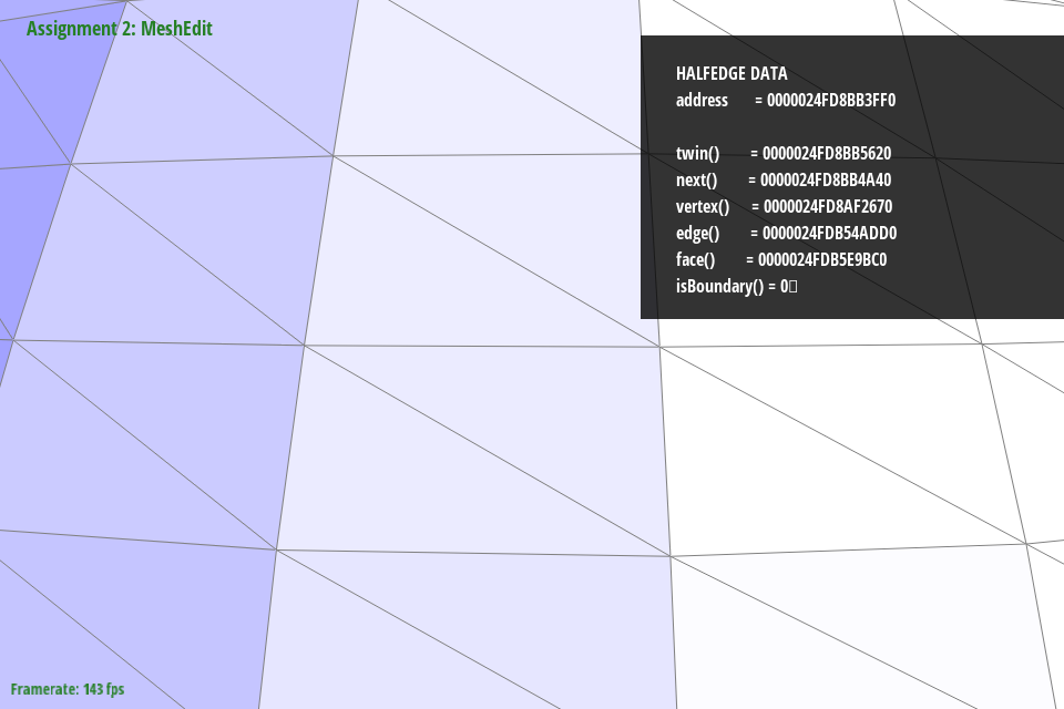 Figure 15: teapot.dae with no edge flips |
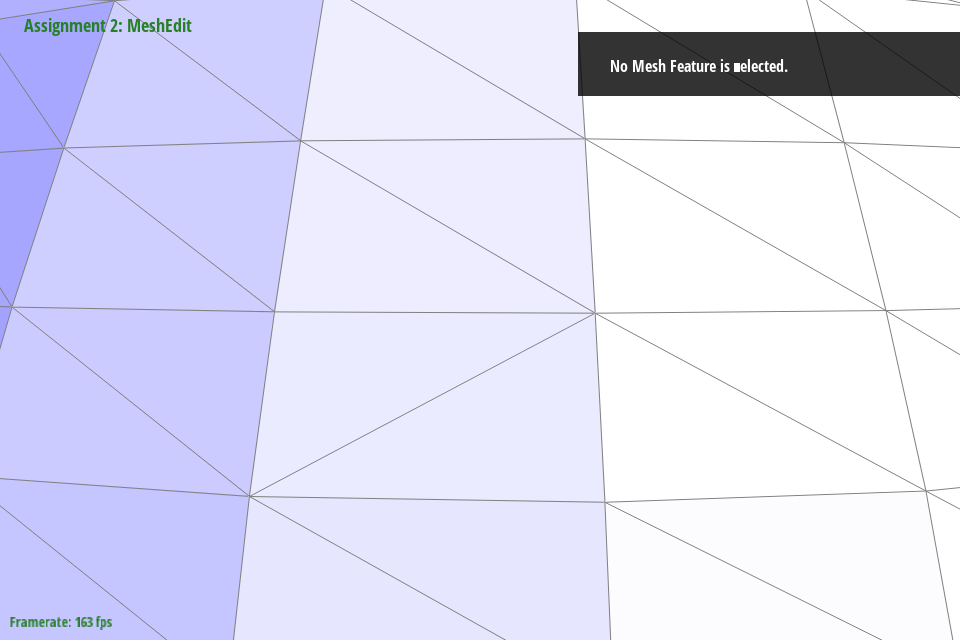 Figure 16: teapot.dae with one diagonal edge flip |
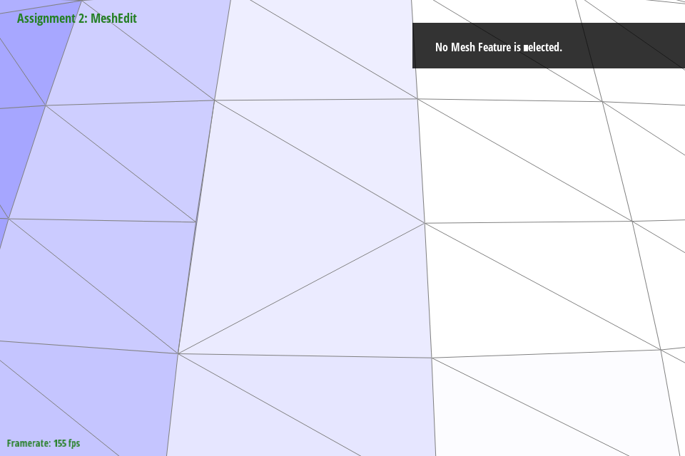 Figure 17: teapot.dae with one diagonal edge flip and one horizontal edge flip |
Edge splitting is the process by which we split the one fully enclosed edge within a mesh into two, thereby creating four faces from two existing faces. The process for accomplishing this is much the same as with edge flipping in that pointers must be modified in order to signify that edges and vertices have moved. Unlike edge flipping, however, we must add components to the mesh. That would be: 2 edges (4 half-edges), 1 face, and 1 vertex per split.
We begin by creating a new vertex that is halfway between the existing two vertices bounding the original passed edge $e_0$. Note that in the code this is renamed to $e_{0n}$. This is to better match the naming schema (explained later in this response), however any mention of $e_0$ is equivalent to $e_{0n}$ and vice versa.
The image below, copied from part 4, shows the edges $e_X$, half-edges $h_X$, vertices $v_X$, and faces $f_X$ of a singular example mesh.

Figure 18: Triangle mesh with labeled components
Following the retrieval of all these components, we then create the new components. This is done using newHalfedge(), newEdge(), newFace(), and newVertex() for halfedges, edges, faces, and vertices respectively. When created, these objects come with no properties filled and as such must be updated (much as in part 4).
The image below (now different from part 4) shows what a mesh should look like after an edge in that mesh has been split. The naming schema of using $h_{Xt}$ for edges twinned to $h_X$ returns from part 4. In addition, we add the $h_{0n/s/e/w}$ nomenclature. This is to distinguish which cardinal direction a half-edge is pointing from the newly created center vertex. The 0 is included to note that this is a product of the original halfedge $h_0$. We assign $h_0$ to $h_{0n}$ so as to not discard halfedges unnecessarily (i.e. use unnecessary additional resources). Edges are named in accordance with this cardinality-defined halfedge schema (for example, halfedges $h_{0s}$ and $h_{0st}$ are along edge $e_{0s}$. The center vertex is not denoted as $v_0$ (instead incrementing on the previous maximum to $v_4$) to maintain vertex placement with the previous parts.
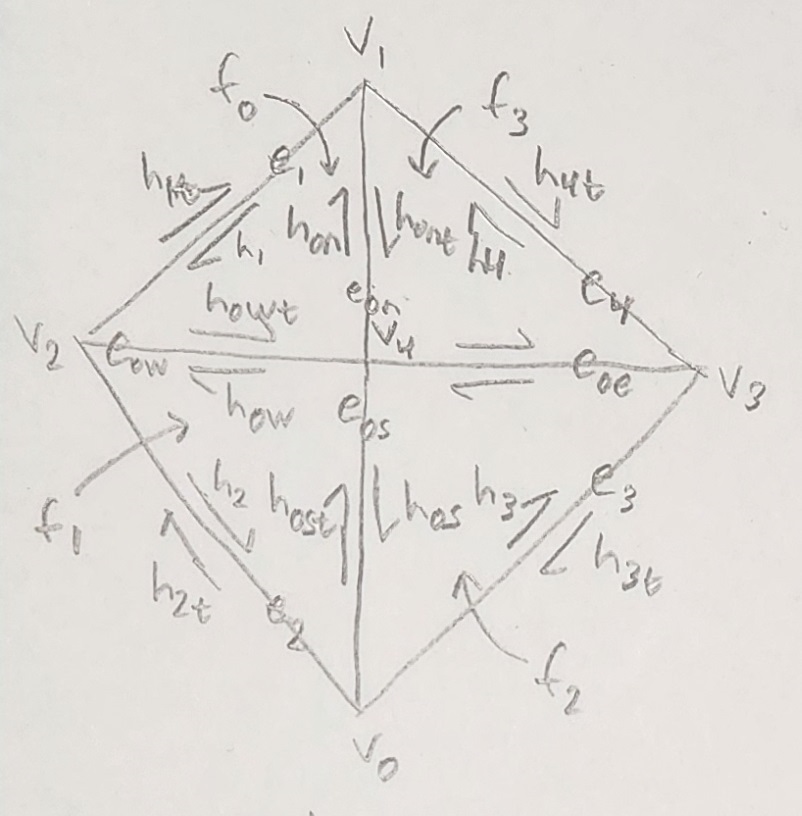
Figure 19: Triangle mesh with labeled components after edge split
As with part 4, we can ignore the neighbors of the outer halfedges since they will continue to connect to other external components. However, unlike part 4 we cannot assume that this means all twinned halfedges do not need to be modified. Because we are creating new halfedges for the inner edges, the neighbors of these twinned halfedges must be assigned in addition to the other inner halfedges.
Again in keeping with part 4, we must also assign halfedges to edges. These may be chosen arbitrarily between an edge or its twinned edge, though for the sake of debugging they are the primary (i.e. nontwinned) halfedges. Faces are similarly arbitrarily assigned any halfedge contained within itself.
The primary difference with splitting edges is that we must mark some edges as “new” by setting the isNew flag to true. These edges are $e_{0e}$ and $e_{0w}$ (in addition to the center vertex $v_4$. We do not mark the edge $e_{0s}$ as new despite it being newly created since it occupies a portion of the original $e_0$ edge. $e_{0n}$ is also excluded for the same reason, though in code we additionally denote that the original $e_0$ is sized down to $e_{0n}$ while $e_{0s}$ is created to replace the line segment freed by resizing $e_0$ to $e_{0n}$.
The position of the newly created vertex is the midpoint of the original edge $e_0$. This position is retrieved by adding the positions of the vertices from which the halfedges $h_0$ and $h_{0t}$ originate, i.e. the end vertices of the edge $e_0$. Divide this by two to get the midpoint. In our case we multiply by 0.5 since multiplication is a much faster operation than division.
The return value of the function is then the newly created vertex $v_4$.
While debugging this part was largely the same as part 4 in that we looked primarily at the mesh properties in the GUI. The below is copied from part 4 since it also applies here:
“By noting the address and comparing it to other objects, we could see where pointers were being assigned and if they were being assigned correctly. As a trick to make debugging faster, we truncated addresses to the last 4 digits since most components around a mesh seemed to be unique in that address space. Originally we tried with 3, but that led to some components being mistaken for each other that were in fact distinct in the fourth digit. We also ended up using temporary variables to store all halfedges, twinned halfedges, faces, edges, and vertices following my naming format outlined above. This saved debugging time by making it significantly easier to spot neighbor assignment issues just from looking at variable names.”
The images below show an example teapot.dae model with (1) no edge splits, (2) one edge diagonal edge split, and (3) one diagonal edge split and one horizontal edge split.
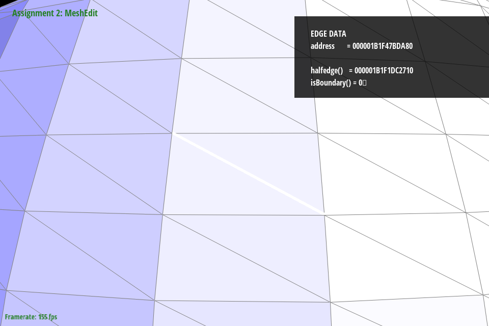 Figure 20: teapot.dae with no edge splits |
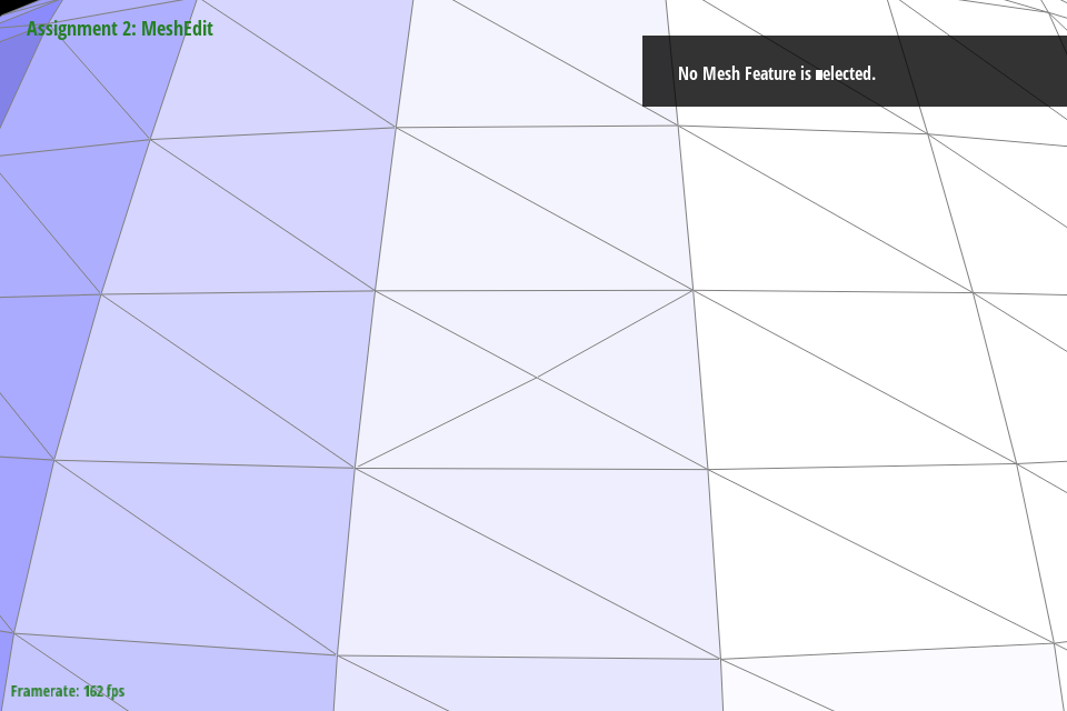 Figure 21: teapot.dae with one diagonal edge split |
 Figure 22: teapot.dae with one diagonal edge split and one horizontal edge split |
When put in combination with edge flips, we get two very different behaviors. If a split is performed before a flip, the edge that is flipped will likely disappear. This of course depends on the geometry of the part, but for this we assume we have a fairly normal rectangular mesh. If a flip is performed before a split, we get the same outcome as a normal split. This makes sense intuitively, as a flip means the inner edge splits vertices within the mesh, but a split will reconnect the previously disconnected vertices with a new edge.
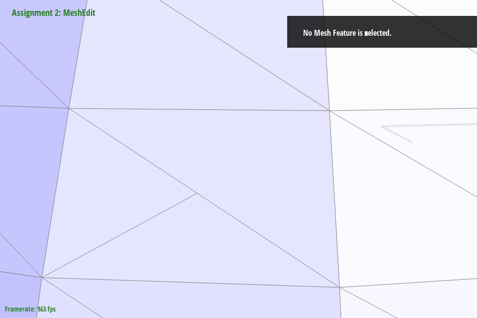 Figure 23: teapot.dae with a split then a flip |
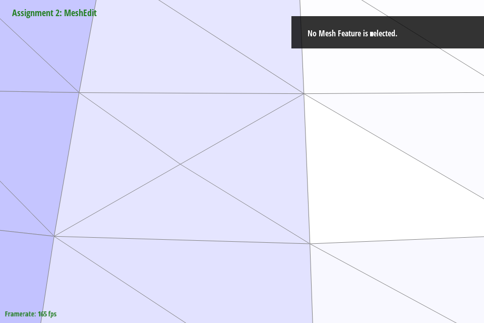 Figure 24: teapot.dae with a flip then a split |
In our original implementation of edge splitting, we had a check to immediately return a blank dummy vertex if the original edge $e_0$ was a boundary edge. However, we should support being able to split on boundary edges as they appear frequently, for example in beetle.dae (which is a model of a VW Beetle body). Support for boundary splitting is implemented in place of this previous check for a boundary edge.
As with the first portion of part 5, we start by drawing out a mesh and its components. This ends up looking like the image below. Observe that the boundary halfedge is $h_{0t}$. The reasoning for making this $h_{0t}$ and not $h_0$ is that the passed edge originates at $v_0$ and as such it is an inner halfedge. This is by design such that we again have $h_X$ on the inner halfedges and $h_Xt$ on the outer halfedges. The dashed lines indicate the other neigboring meshes on the left and the hole/empty space on the right.
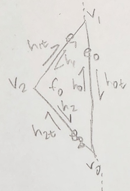
Figure 25: Triangle mesh with boundary edge and labeled components
When performing an edge split on this outer edge $e_0$ we then only need to create half the mesh components of the original operation. A visualization of this is shown below, totaling 1 face, 1 vertex, 2 edges, and 4 halfedges.
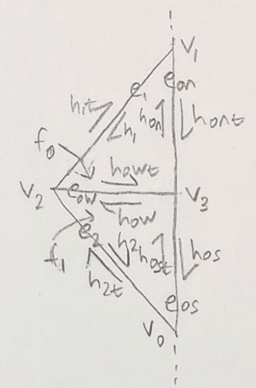
Figure 26: Triangle mesh with boundary edge and labeled components after split
Again like the first portion of part 5, we assign neighbors for each of the inner halfedges, assign halfedges to edges, and assign halfedges to faces. Only one edge, the one connecting $v_2$ to the newly created vertex $v_3$, is marked as new (in addition to said vertex). Vertex $v_3$ is denoted as $v_3$ instead of the previous $v_4$ because there is now one fewer vertex in the mesh object.
When assigning the next() halfedges, we must be careful that we assign the correct halfedges to the outer halfedges. In more detail, since the outer halfedge $h_{0t}$ is not made part of any new component it must retain its connection to its next() halfedge and the face it is a part of. To do this we resize $h_0t$ to connect $v_1$ to the midpoint $v_4$, then add a new halfedge $h_{0s}$ to connect $v_4$ to $v_0$, the original endpoint of $h_{0t}$. Thus the next() of $h_0nt$ is $h_{0s}$ and the next() of $h_{0s}$ is the original next() for $h_{0t}$. Similarly, both maintain the same face as $h_{0t}$ (now $h_{0nt}$).
The four images below show this functionality working to split a boundary edge: (1) with no boundary split, (2) with one boundary split, (3) with two boundary splits, and (4) with three boundary splits.
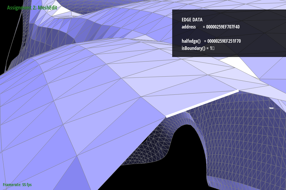 Figure 27: beetle.dae with no edge splits |
 Figure 28: beetle.dae with one edge split |
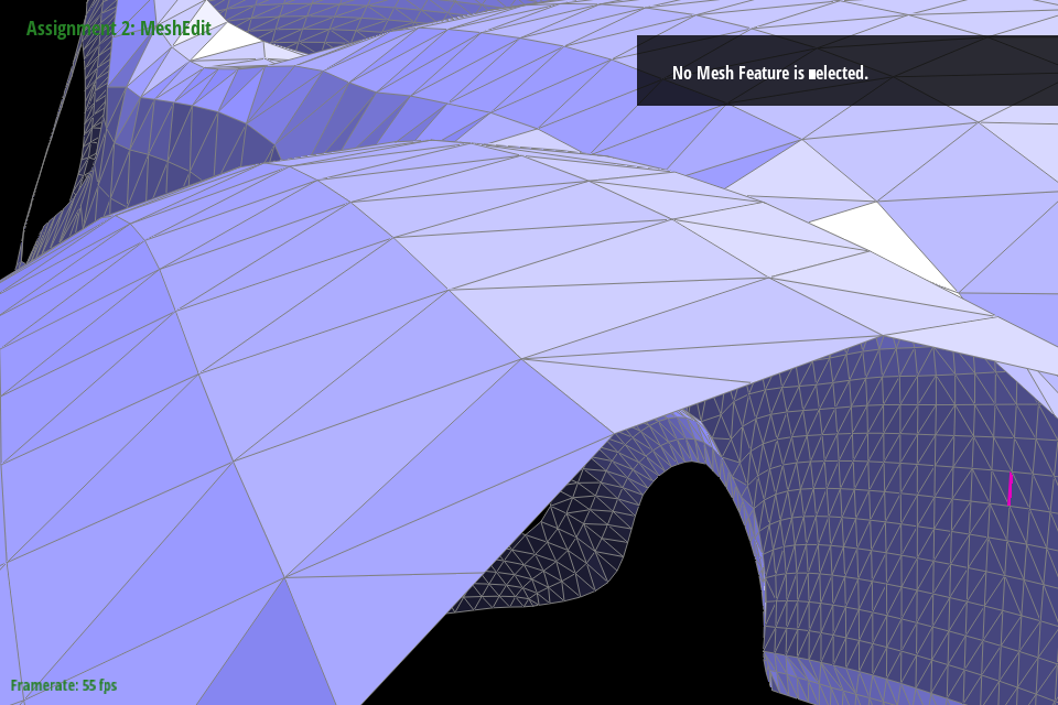 Figure 29: beetle.dae with two edge splits |
 Figure 30: beetle.dae with three edge splits |
Loop subdivision is the process by which we split every triangle then weight the positions of the vertices by some amount. Notably, this exercise uses the splitting and flipping functionality of both part 4 and part 5. To implement this, we follow a basic procedure:
- Compute the positions of the new and old vertices
- Subdivide the mesh by splitting and flipping
- Update the new vertex positions to the calculated positions
As noted in the spec, we perform the mesh manipulation in this order to traverse a minimum number of elements (i.e. avoid traversing the split and flipped mesh with significantly more elements).
To compute the new positions of the edges, we iterate through every edge in the mesh and set the newPosition of the iterative edge to $\frac{1}{8}(v_a+v_b)+\frac{3}{8}(v_c+v_d)$. $v_a$ and $v_b$ are vertices associated with the halfedge assigned to the current edge $h_0$ and its twin $h_{0t}$. $v_c$ and $v_d$ are the two remaining vertices, which are retrieved by following the next() pointers twice and using the assigned vertices.
After computing the new edge positions we compute the new vertex positions. These vertex positions are a function of the sum of their neighbors’ positions. This variable, called original_neighbor_position_sum, is a Vector3D which is the sum of positions for each vertex neighbor, iterated through by halfedge. The vertex positions are then (as denoted in the spec) a function of n (the degree of the vertex, which should not change) and u (a weighting term). u is set to $3/16$ if $n == 3$ is true, or $3/(8n)$ otherwise. Again as denoted in the writeup, the new position of the vertex is (1 - n * u) * original_position + u * original_neighbor_position_sum.
We then perform the splitting and flipping operations (in that order) per edge. We can combine these two operations into the same iterative loop as a flip will not influence the external connections of any given mesh. As we iterate through the edges, only edges that have two old vertices are split. Equivalently, edges which are composed of one or more newly created edges (for example, from splitting) are not split. Similarly, only new edges which have one old and one new vertex are then flipped. This is an XOR operation, which is implemented very eloquently in C with (v0->isNew + v1->isNew) == 1. This operation interprets the boolean isNew values into 1 for true or 0 for false, then adds them together. Thus, only if one of them is true will they be equal to 1.
Finally, we iterate through each vertex in the split mesh and assign the vertex’s official position to its newPosition. We also mark these vertices as old by setting isNew to false for all edges.
In general, the effect of loop subdivision is to make meshes composed of triangles smoother. This smoothing comes from the weighting of the edges, and the additional edges which allow a finer grain of control especially with surfaces that should be smooth. That being said, surfaces which should be pointy are made smooth incorrectly when loop subdividing. To address this with a known surface, you could pre-split the surfaces which are not on corners/edges (i.e. the diagonal edges of each face of a cube). This would reduce the effective available smoothing area of the upscaling operations.
 Figure 31: teapot.dae with no upscaling |
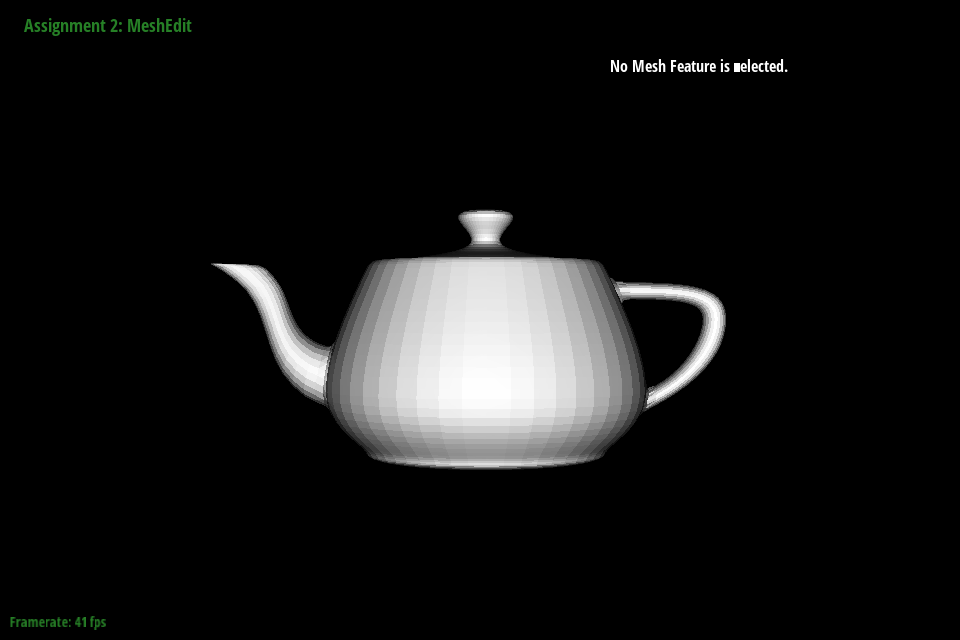 Figure 32: teapot.dae with one level of upscaling |
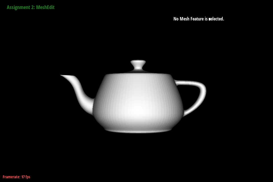 Figure 33: teapot.dae with two levels of upscaling |
 Figure 34: teapot.dae with no upscaling (wireframe) |
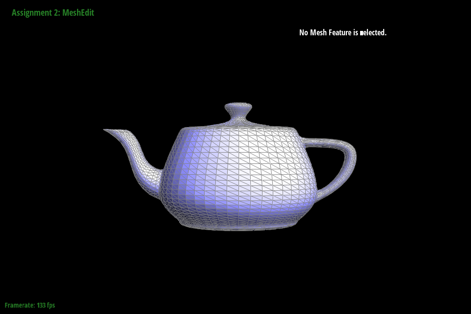 Figure 35: teapot.dae with one level of upscaling (wireframe) |
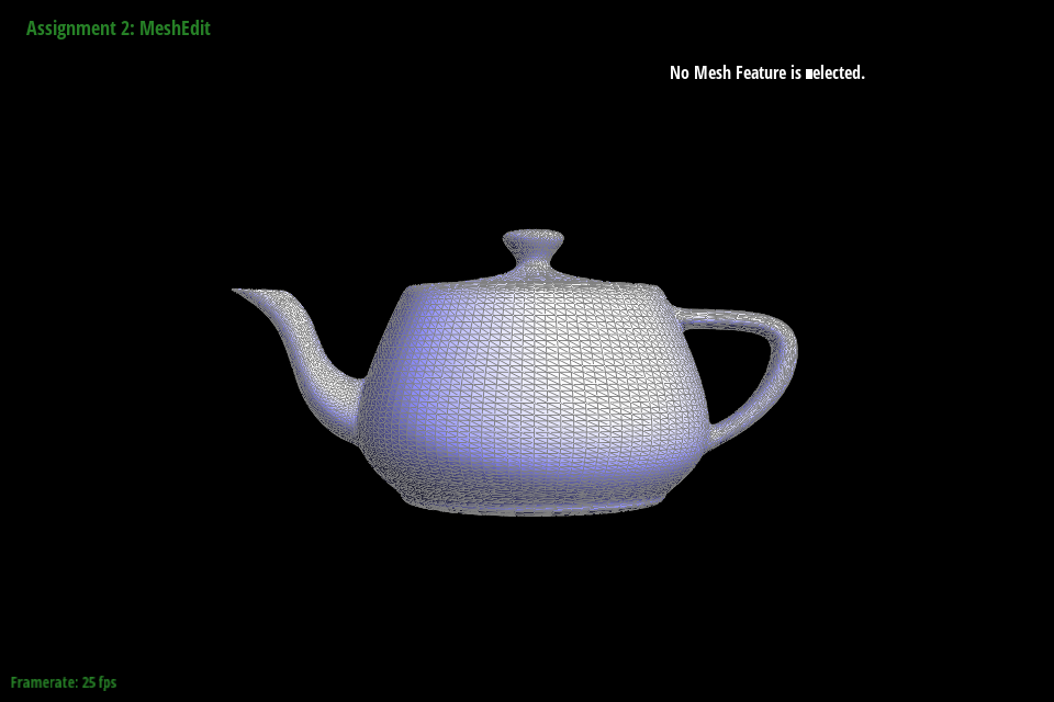 Figure 36: teapot.dae with two levels of upscaling (wireframe) |
Similarly, to split a cuboid object symmetrically you could treat the corner edges as boundary edges (or at a simpler level just the corner vertices). That would preserve the edges and the symmetry of the edges while also not weighting said sharp edges against other subdivided points (such as the newly created inner vertex on each face after being split). This could also be contributed to by the ordering of vertex splitting being performed on one side first, then continuing over the whole mesh. You could do a similar operation to the above teapot where you pre-split the inner edges first to reduce the available effective smoothing area of corner upscaling.
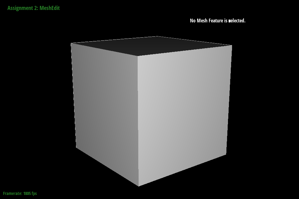 Figure 37: cube.dae with no upscaling |
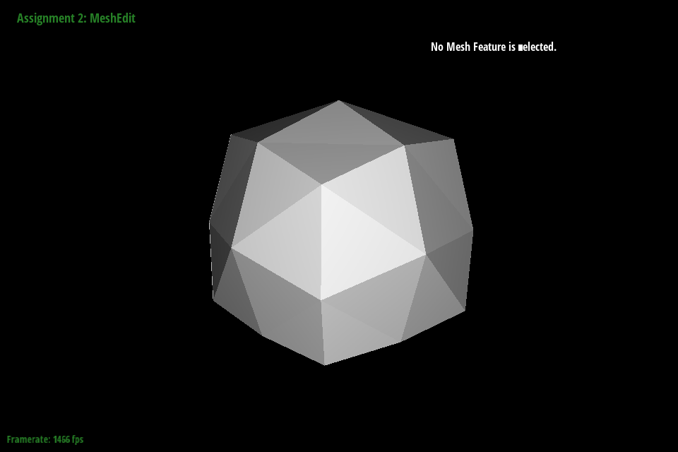 Figure 38: cube.dae with one level of upscaling |
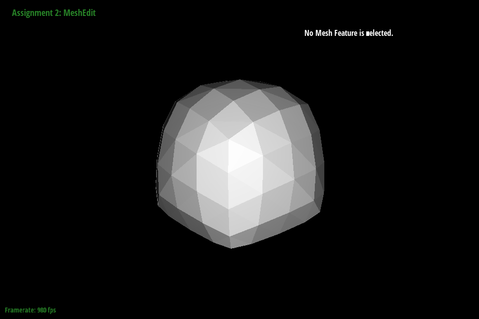 Figure 39: cube.dae with two levels of upscaling |
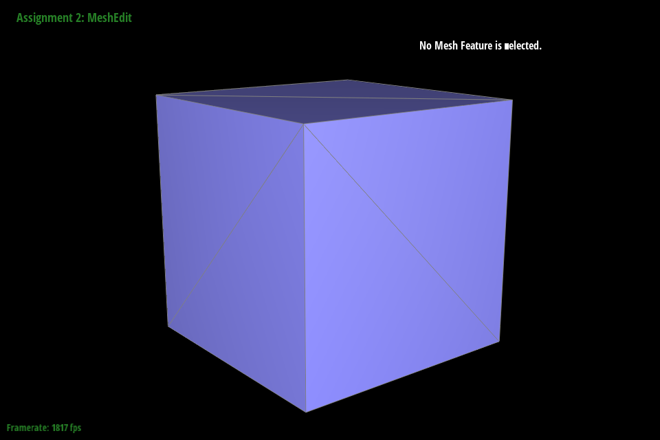 Figure 40: cube.dae with no upscaling (wireframe) |
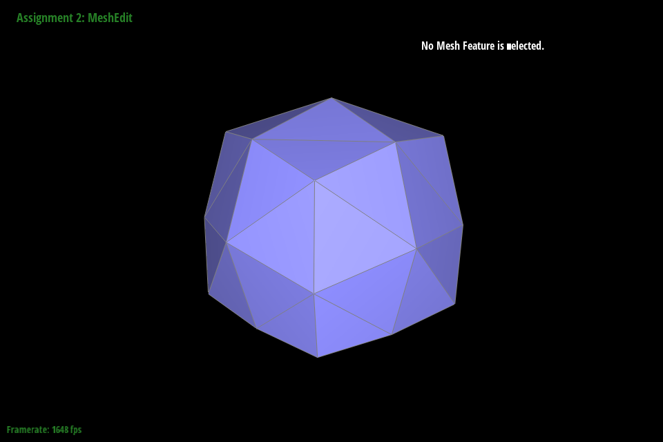 Figure 41: cube.dae with one level of upscaling (wireframe) |
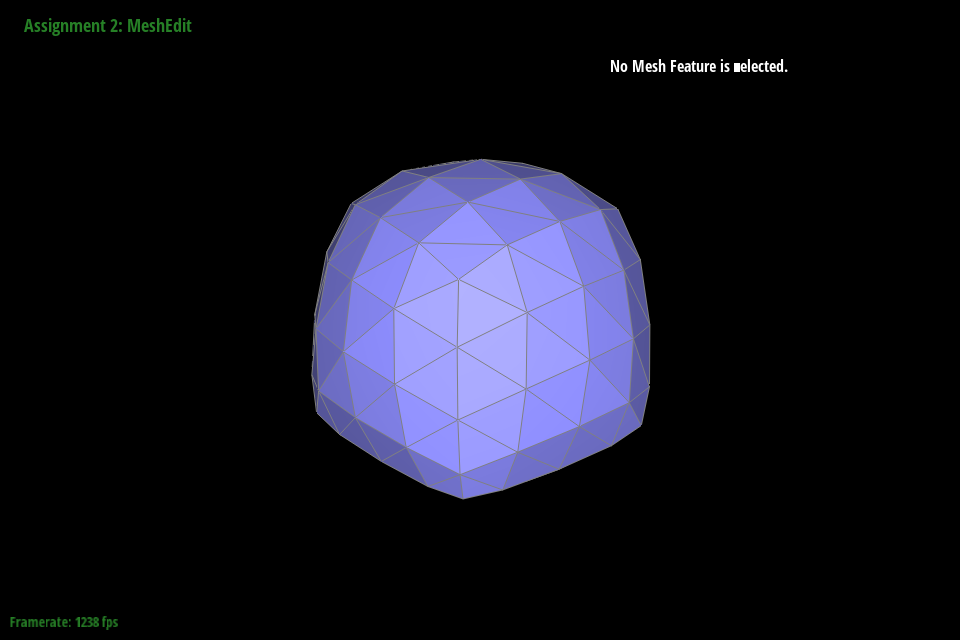 Figure 42: cube.dae with two levels of upscaling (wireframe) |
To implement loop subdivision on meshes with boundary edges, we first have to allow splitting for boundary edges. This is an extra credit for part 5, and as such is documented there. Suffice it to say here that boundary edge splitting works.
We then need to determine how to change the weighting of the vertices and edges such that boundary edges are supported. Referencing the paper linked in the spec, the new position of a vertex is $\frac{3}{4}v_0+\frac{1}{8}(v_1+v_2)$. The original vertex is $v_0$ and its two neighbors are $v_1$ and $v_2$, retrieved by pointer traversal in halfedges. Edge weighting follows from the idea that there are now only two neighbors to a boundary edge, i.e. $(1/2)(v_a+v_b)$. We can furthermore move the extraction of $v_c$ and $v_d$ into a conditional block that requires a non-boundary edge to save computation in the boundary edge case. Both of these modifications are in addition to normal non-boundary edge position calculation, so they require conditionals to check the isBoundary() property.
The result of this is that models with boundary edges subdivide and upscale in the same fashion as models without boundary edges. An example of that is shown below with the beetle.dae model
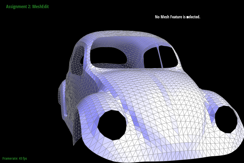 Figure 43: beetle.dae before subdivision |
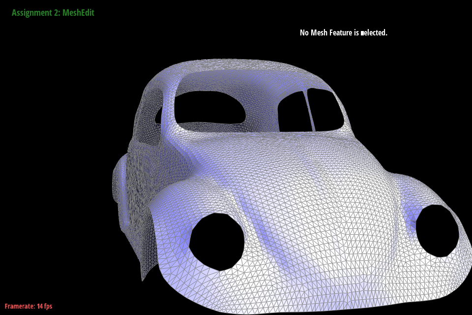 Figure 44: beetle.dae after subdivision |
Chunky cat is a 3D model of a cat that we created by using the software Blender. We first started with a cube that was sculpted into the body and legs, and then we added the head, ears, and tail. These components were formed by extruding faces and moving edges and vertices in the mesh. To add more detail, loop cuts were applied to divide the mesh which allowed more faces to extrude and sculpt. Finally, the features were refined by smoothing the lines to give curves to the original sharp rectangular shapes, carving out the cat's round belly and arched tail.
Each round of subdivision smooths the edges and makes some features less prominent, especially the ears and the paws.
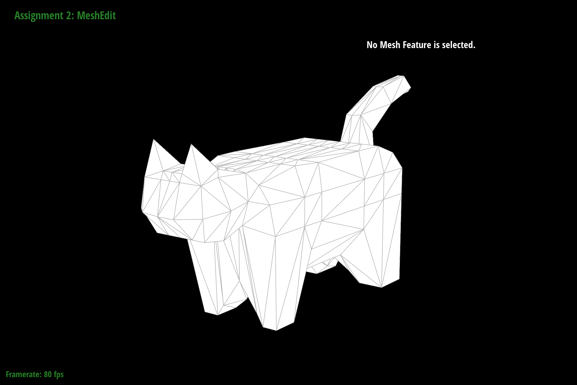 Figure 45: artcompetition.dae with no upscaling |
 Figure 46: artcompetition.dae with one level of upscaling |
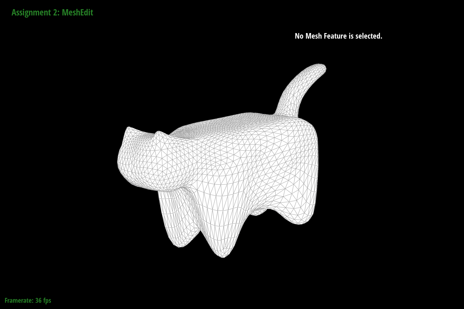 Figure 47: artcompetition.dae with two levels of upscaling |