Homework1 ↵
Homework 1: Rasterizer Overview
Overview
In this homework, we implement a rasterizer that:
- Able to rasterize triangles, points and lines
- Support supersampling
- Support multiple sampling techniques: nearest and bilinear
- Support level sampling
- Support multiple level sampling techniques: level 0, nearest and interpolation
We also implement the translation, scaling and rotation of SVG elements, and created our own SVG robot figure.
We build up our documentation website using markdown and GitHub Pages. Which is the site(or the PDF file) you are currently viewing. We add navigation bar, table of contents, code syntax highlighting and many other details to make the website more readable.
You can find the detailed implementation and explanation of each task in the following pages. Happy reading!
Note for PDF
Some features of the website, such as picture lightbox, may not be available in the PDF version. We recommend reading the website directly for the best experience.
Task 1: Drawing Single-Color Triangles
Method
The high-level idea of drawing triangles comes in two steps:
-
Bounding Box: Find the bounding box of the triangle, which is the smallest rectangle that contains the triangle. This is done by finding the minimum and maximum x and y coordinates of the triangle.
-
Rasterization: For each pixel in the bounding box, check if it is inside the triangle. If it is, color it with the triangle's color.
Implementation
Bounding Box
Given the three vertices of the triangle, finding x limits and y limits is straightforward. However, the limits are not necessarily integers. In order to ensure the bounding box fully covers the triangle, we need to take the ceiling and floor of the limits. To elaborate, the x minimum and y minimum should be rounded down when finding the boundary pixels, vice versa.
    // Step 1: Find the bounding box of the triangle
    // The bounding box should at least cover the triangle, so for the left side, we take the floor of the minimum x coordinate of the triangle
    int bounding_box_x_min = (int)floor(min(x0, min(x1, x2)));
    // For the right side, we take the ceiling of the maximum x coordinate of the triangle
    int bounding_box_x_max = (int)ceil(max(x0, max(x1, x2)));
    // The same implementation for the y coordinate--floor for the bottom and ceiling for the top
    int bounding_box_y_min = (int)floor(min(y0, min(y1, y2)));
    int bounding_box_y_max = (int)ceil(max(y0, max(y1, y2)));
Rasterization
Implicit line equations are implemented to determine whether a sample position is inside or on the edge of the triangle:
If \(P_0(x_0,y_0)\) and \(P_1(x_1,y_1)\) are two points on the line, then \(dX = x_1 - x_0\), \(dY = y_1 - y_0\).
If \(L\) yields all positive results for the three edge, then the sample position is considered inside the triangle. When \(L = 0\), the sample position is on the edge. Both situations the sample position should be colored.
Through the above method, each pixel's color could be determined through a one-time iteration.
    // Step 2: Iterate through all the pixels in the bounding box
    // Initializing variables
    int current_x_position, current_y_position;
    float line01_delta_x = x1 - x0;
    float line01_delta_y = y1 - y0;
    float line12_delta_x = x2 - x1;
    float line12_delta_y = y2 - y1;
    float line20_delta_x = x0 - x2;
    float line20_delta_y = y0 - y2;
    float line01_result, line12_result, line20_result;
    // iterate through lines
    for (current_y_position = bounding_box_y_min; current_y_position < bounding_box_y_max; current_y_position++)
    {
        // iterate through pixels in the line
        for (current_x_position = bounding_box_x_min; current_x_position < bounding_box_x_max; current_x_position++)
        {
          // check if the pixel is inside the triangle. If so, fill the corresponding buffer
          // note when calculating line results, we should use the CENTER of the pixel as position
          line01_result = - ((float)current_x_position + 0.5 - x0) * line01_delta_y + ((float)current_y_position + 0.5 - y0) * line01_delta_x;
          line12_result = - ((float)current_x_position + 0.5 - x1) * line12_delta_y + ((float)current_y_position + 0.5 - y1) * line12_delta_x;
          line20_result = - ((float)current_x_position + 0.5 - x2) * line20_delta_y + ((float)current_y_position + 0.5 - y2) * line20_delta_x;

          if (line01_result >= 0. && line12_result >= 0. && line20_result >= 0.)
          {
            fill_pixel(current_x_position,current_y_position,color);
          }
        }
    }
Results
The following image is the rasterized result of basic/test4.svg:

Task 2: Antialiasing by Supersampling
Method
In task 2, antialiasing is implemented by supersampling and downsampling. The main steps involves:
-
Creating and maintaining sample buffer: To store the supersampling result, a sample buffer corresponding to the sample rate is created and managed throughout the render pipeline. When sample rate updates, the sample buffer should be updated accordingly.
-
Supersampling with sample buffer: Sampling the triangle implements the sample buffer with the same method as in task 1 except the vertice position of triangle should be transformed to the sample buffer coordinate. However, lines and points should not be antialiased. They need to be zoomed in by the sample rate before populating the sample buffer.
-
Downsampling and populating frame buffer: Downsampling the sample buffer to the frame buffer by mixing the color of the samples corresponding to the same pixel.
Implementation
Creating and maintaining sample buffer
When the sample rate is updated, sample buffer should be resized. As RasterizerImp::set_sample_rate updates sample rate, the buffer is resized when the function is called:
  void RasterizerImp::set_sample_rate(unsigned int rate)
  {
    // TODO: Task 2: You may want to update this function for supersampling support

    this->sample_rate = rate;

    // updated for supersampling
    this->sample_buffer.resize(width * height * sample_rate, Color::White);
  }
The same applies to RasterizerImp::set_framebuffer_target:
  void RasterizerImp::set_framebuffer_target(unsigned char *rgb_framebuffer,
                                             size_t width, size_t height)
  {
    // TODO: Task 2: You may want to update this function for supersampling support

    //cout << "set_framebuffer_target" << endl;

    this->width = width;
    this->height = height;
    this->rgb_framebuffer_target = rgb_framebuffer;

    //updated for supersampling
    this->sample_buffer.resize(width * height * sample_rate, Color::White);
  }
Supersampling with sample buffer
Define \(zoom\_coefficient = \sqrt{sample\_rate}\), the transformation of the vertice position of triangle to the sample buffer coordinate is:
    // Step 1: Convert the triangle vertices to the supersample buffer's coordinate system
    int zoom_coefficient = sqrt(sample_rate);
    float x0_ss = x0 * zoom_coefficient;
    float y0_ss = y0 * zoom_coefficient;
    float x1_ss = x1 * zoom_coefficient;
    float y1_ss = y1 * zoom_coefficient;
    float x2_ss = x2 * zoom_coefficient;
    float y2_ss = y2 * zoom_coefficient;
The sampling process is exactly the same as in task 1, except the result fills sample buffer instead of frame buffer.
For lines and points, they fill directly to the frame buffer pixels. This can be achieved by filling all the subpixels in the sample buffer with the same color. These subpixels form a square of size \(zoom\_coefficient \times zoom\_coefficient\). A double loop is implemented to iterate all the subpixels.
  void RasterizerImp::fill_pixel(size_t x, size_t y, Color c)
  {
    // TODO: Task 2: You might need to this function to fix points and lines (such as the black rectangle border in test4.svg)
    // NOTE: You are not required to implement proper supersampling for points and lines
    // It is sufficient to use the same color for all supersamples of a pixel for points and lines (not triangles)

    // Implementation by Ruhao Tian starts here
    // As points and lines are not required to be supersampled, we can simply fill the corresponding buffer with given color
    int zoom_coefficient = sqrt(sample_rate);
    for (int i = 0; i < zoom_coefficient; i++)
    {
      for (int j = 0; j < zoom_coefficient; j++)
      {
        sample_buffer[(y * zoom_coefficient + j) * width * zoom_coefficient + x * zoom_coefficient + i] = c;
      }
    }
  }
Downsampling and populating frame buffer
RasterizerImp::resolve_to_framebuffer resolves the sample buffer to the frame buffer. It iterates all the pixels in the frame buffer. For each pixel, its subpixel square is located.
The R, G, B values of all subpixels are averaged respectively and assigned to a temporary Color object ds_color:
        // for each pixel, calculate the average color of all the samples
        ds_color.r = 0;
        ds_color.g = 0;
        ds_color.b = 0;

        for (int i = 0; i < zoom_coefficient; i++)
        {
          for (int j = 0; j < zoom_coefficient; j++)
          {
            ds_color.r += sample_buffer[(y * zoom_coefficient + j) * width * zoom_coefficient + x * zoom_coefficient + i].r / (float)(sample_rate);
            ds_color.g += sample_buffer[(y * zoom_coefficient + j) * width * zoom_coefficient + x * zoom_coefficient + i].g / (float)(sample_rate);
            ds_color.b += sample_buffer[(y * zoom_coefficient + j) * width * zoom_coefficient + x * zoom_coefficient + i].b / (float)(sample_rate);
          }
        }
Then the conversion of ds_color to rgb_framebuffer_target is the same as base code:
        for (int k = 0; k < 3; ++k)
        {
          this->rgb_framebuffer_target[3 * (y * width + x) + k] = (&ds_color.r)[k] * 255;
        }
The full implementation of RasterizerImp::resolve_to_framebuffer is:
  void RasterizerImp::resolve_to_framebuffer()
  {
    // TODO: Task 2: You will likely want to update this function for supersampling support

    // Implementation by Ruhao Tian starts here

    //cout << "resolve_to_framebuffer" << endl;

    int zoom_coefficient = sqrt(sample_rate);
    Color ds_color(0, 0, 0);

    for (int x = 0; x < width; ++x)
    {
      for (int y = 0; y < height; ++y)
      {
        // for each pixel, calculate the average color of all the samples
        ds_color.r = 0;
        ds_color.g = 0;
        ds_color.b = 0;

        for (int i = 0; i < zoom_coefficient; i++)
        {
          for (int j = 0; j < zoom_coefficient; j++)
          {
            ds_color.r += sample_buffer[(y * zoom_coefficient + j) * width * zoom_coefficient + x * zoom_coefficient + i].r / (float)(sample_rate);
            ds_color.g += sample_buffer[(y * zoom_coefficient + j) * width * zoom_coefficient + x * zoom_coefficient + i].g / (float)(sample_rate);
            ds_color.b += sample_buffer[(y * zoom_coefficient + j) * width * zoom_coefficient + x * zoom_coefficient + i].b / (float)(sample_rate);
          }
        }

        for (int k = 0; k < 3; ++k)
        {
          this->rgb_framebuffer_target[3 * (y * width + x) + k] = (&ds_color.r)[k] * 255;
        }
      }
    }

    //cout << "resolve_to_framebuffer done" << endl;
  }
Results
The following images are the result of supersampling basic/test4.svg with sample rates 1, 4 and 16.
Image displayed size too small?
Click on the image to activate lightbox mode. In lightbox mode, click on the arrows on the left and right to navigate through images. This brings easy comparison.


The following images show a zoomed view of one triangle in basic/test4.svg. The left image is the result of sample rate 1 while the other one implements sample rate 16.


In the left image, the top of the triangle seemed 'disconnected' from the other part. This is because, in the disconnected part, all the nearby sample points(center of pixels) are outside the triangle. When the sample rate increases, the subpixels inside the triangle are identified. This comparison shows the effectiveness of supersampling in antialiasing--it not only smooths the edges but also corrects the display of the image.
Task 3: Transforms
SVG Design
The overall idea is to design a robot with black hair, yellow skin, grey trousers and a T-shirt with Berkeley's iconic orange and blue color. The posture of robot is standing with right arm on the waist and left arm waving.
Setting up colors
With the help of palette software, the RGB code of colors is obtained:
- Black: #000000
- Yellow: #f3cb81
- Grey: #353535
- Orange: #e09811
- Blue: #0b106e
Filling the colors in the SVG file, the robot is rendered as follows:

Transforms
The right arm of the robot is rotated by -45 degrees, the forearm is rotated by -90, and the relative position is slightly adjusted:(modifications are highlighted in the code below)
The left big arm and forearm of the robot are rotated by -45 degrees, their relative position is adjusted as well:
The robot is rendered as follows:

Task 4: Barycentric coordinates
Methodology
The Barycentric Coordinate System
The barycentric coordinate presents a point in a triangle with the weighted sum of the triangle's vertice positions. Assume triangle vertices \(A(x_{A},y_{A})\), \(B(x_{B},y_{B})\), and \(C(x_{C},y_{C})\), position of any point \(P(x_{P},y_{P})\) inside the triangle can be calculated as:
where \(\alpha + \beta + \gamma = 1\). In other words, \(\alpha\), \(\beta\) and \(\gamma\) are the weights showing how much each vertex contributes or is close to the point \(P\).
Calculation
One way to represent how close a point is to a vertex is to calculate its proportional distance to the edge opposite to the vertex, as is shown in the following figure:

Assume \(D_{BC}\) to be the distance to edge \(BC\), the \(\alpha\) weight can be calculated as:
Point-to-line distance formula can be used to calculate \(D\):
Replace \(D_{BC}\) in the \(\alpha\) formula, we get:
Similarly, \(\beta\) and \(\gamma\) can be calculated as:
Features of Barycentric Coordinates
The Barycentric coordinates' distinctive feature makes it suitable for geometric calculations in computer graphics. This includes but is not limited to:
- Interpolation: Barycentric coordinates can be used to interpolate values smoothly varying across a triangle. This is useful in texture mapping, color blending, and shading.
- Invariance to affine transformations: Regardless of the affine transformation applied to the triangle, the relative position of the vertices remains the same. As Barycentric coordinates are based on the relative position of the vertices, it could simplify calculation when affine transformations are involved.
Implementation
To determine whether a point is inside a triangle with Barycentric coordinates, whether the three weights are all positive is the only thing needed to check. For the points inside the triangle, its color is the weighted sum of the triangle's vertices' color, where the weights are exactly the Barycentric coordinates' weights. Other parts of the rasterization process are the same as Task 2.
The following code shows the rasterization process with Barycentric coordinates, highlighted are the parts where Barycentric coordinates are involved:
Results
The screenshot of svg/basic/test7.svg is shown below.

Task 5: "Pixel sampling" for texture mapping
Methodology
Texture Coordinates Mapping

Given an unfolded texture image and a 3D model, the mission is to 'wrap around' the texture onto the 3D model. During this process, the 2D texture image is divided into many triangles, each of which corresponds to a triangle on the 3D model. However, the 3D model has a different coordination system from the 2D image. Therefore, texture coordinates mapping is needed to map the 2D texture image to the 3D model.
As discussed in the previous task, the Barycentric coordinates remain the same however the triangle transforms affinely. Therefore, given a point on the 3D model, one can obtain its matching point on the 2D texture by finding out its Barycentric coordinates and then using the Barycentric coordinates to interpolate the texture coordinates. This lays the foundation for texture mapping.
Pixel Sampling
Pixel sampling finds which color should be displayed on the screen pixel. First, the corresponding point on the 3D model of the pixel sample point is found, which is the job of the rasterizer. As the color of the triangle is decided by its texture, the next step is to find the corresponding color point on the texture. After that, the color is returned all the way back to the pixel point. This whole process is described in the following figure.
flowchart TB
  A[Start:
  Sample Point
  in screen space]
  B[Rasterizer:
  Find the corresponding point
  on the 3D model];
  C[Texture Mapping:
  Find the corresponding point
  on the texture]
  A -->|Sample Point Position| B;
  B -->|Barycentric Coordinate Position| C;
  C -->|Color| D[Rasterizer: Get color];
  D -->|Color| E[Screen frame buffer: Get color];
Featured by the density of sample points and texture texels, pixel sampling could be categorized into:
- Magnification pixel sampling: Where texels surplus sample points and each sample point corresponds to several texels. Common sample methods are nearest sampling and bilinear sampling.
- Minification pixel sampling: Where sample points surplus texels and each texel corresponds to several sample points. Common sample methods include mipmap and anisotropic filtering.
Magnification pixel sampling
Nearest sampling
Nearest sampling choose the closest texel to the sample point. Simple idea, low computational complexity, but nearest sampling does not ensure the color of sample pixels will change smoothly, so aliasing is common for nearest sampling.
Bilinear sampling

Bilinear sampling finds 4 closest texels around the sample point. Both horizontal and vertical interpolations are performed to get the final color. Assume \(u_{00}\), \(u_{01}\), \(u_{10}\), \(u_{11}\) are the for texels and \(C\) is the color of texel, the first and second linear interpolation calculate the color of two groups of horizontal texels, based on the proportional distance horizontally sample point is close to the texels:
Then, the final color is calculated by the third linear interpolation, based on the proportional distance vertically sample point is close to the texels:
Bilinear sampling is more complex than nearest sampling, but it can effectively reduce aliasing.
Implementation
Nearest sampling
The nearest texel of the sample point is exactly the texel sample point is in. Therefore, the position of the nearest texel is the integer part of the texture coordinates and can be easily calculated by floor function.
It is worth noting that, as mipmap size varies with the level, the input texture coordinates should be scaled to the mipmap size.
  Color Texture::sample_nearest(Vector2D uv, int level) {
    // TODO: Task 5: Fill this in.
    auto& mip = mipmap[level];


    return mip.get_texel((int)floor(uv.x * mip.width), (int)floor(uv.y * mip.height));
  }
Bilinear sampling
There is a special case for bilinear sampling: when the sample point is so close to the edge of the texture that the position of some closest texels is out of the texture. In this case, the closest texel inside texture is used to replace the out-of-bound texel. In implementation, the position of the out-of-bound texel could be replaced by the position of that closest texel. Take the horizontal direction as an example, the position of out-of-bound texel is replaced by the position of the closest texel inside the texture:
    //find the x coordinate of four nearest texels, as well as the proportion of the distance
    // consider the edge case, if the sample point is on the edge, repeat the nearest texel
    if (uv_x <= 0.5)
    {
      sampletexel_lu[0] = 0;
      sampletexel_ru[0] = 0;
      sampletexel_ld[0] = 0;
      sampletexel_rd[0] = 0;
      // horizontally, the two nearest texels are the same
      x_proportion = 0; // could be any value
    }
    else if (uv_x >= width - 0.5)
    {
      sampletexel_lu[0] = width - 1;
      sampletexel_ru[0] = width - 1;
      sampletexel_ld[0] = width - 1;
      sampletexel_rd[0] = width - 1;

      x_proportion = 0;
    }
    else
    {
      sampletexel_lu[0] = floor(uv_x - 0.5);
      sampletexel_ru[0] = ceil(uv_x - 0.5);
      sampletexel_ld[0] = floor(uv_x - 0.5);
      sampletexel_rd[0] = ceil(uv_x - 0.5);

      x_proportion = (uv_x - 0.5) - floor(uv_x - 0.5);
    }
In the first two situations of if statement, because horizontally the two nearest texels are the same, their weighted color sum will always be the same, which means the proportion of the distance does not need to be calculated and this is why x_proportion is set to 0. In other cases, floor(uv_x- 0.5) gives the left two texels' x coordinates and this coordinate plus by one, equals ceil(uv_x - 0.5)`, giving the right ones. The same logic applies to the vertical direction.
After obtaining the position of the four nearest texels and the proportion of the distance, the color of the sample point is calculated by the formula mentioned above.
    //get the color of four nearest texels
    c_lu = mip.get_texel((int)sampletexel_lu[0], (int)sampletexel_lu[1]);
    c_ru = mip.get_texel((int)sampletexel_ru[0], (int)sampletexel_ru[1]);
    c_ld = mip.get_texel((int)sampletexel_ld[0], (int)sampletexel_ld[1]);
    c_rd = mip.get_texel((int)sampletexel_rd[0], (int)sampletexel_rd[1]);

    //bilinear interpolation
    // first lerp horizontally, then vertically
    temp0 = c_lu * (1 - x_proportion) + c_ru * x_proportion;
    temp1 = c_ld * (1 - x_proportion) + c_rd * x_proportion;
    final = temp0 * (1 - y_proportion) + temp1 * y_proportion;
Results
The following images show the result of nearest sampling and bilinear sampling. From left to right are nearest sampling with supersample rate 1, nearest sampling with supersample rate 16, bilinear sampling with supersample rate 1, and bilinear sampling with supersample rate 16.
Image displayed size too small?
Click on the image to activate lightbox mode. In lightbox mode, click on the arrows on the left and right to navigate through images. This brings easy comparison.


Examine the images, jaggies are visible in the nearest sampling with supersampling rate 16, at the end of "LET THERE BE", which does not appear in bilinear sampling with supersample rate 1.
Discussion
It is clear that bilinear sampling is better than nearest sampling, even bilinear sampling with supersample rate 1 can achieve better results than nearest sampling with supersample rate 16. According to the code, bilinear sampling is certainly more costly, but it smooths the color transition, so images with many high-frequency elements would have a more obvious effect, like this twisted logo with a sharp orange-white transition.
Another noticeable thing is bilinear sampling is more effective than nearest sampling and supersampling combined. This is because supersampling can only smooth the color transition in the pixel level, while bilinear sampling smooths the color transition in the texel level. In magnification pixel sampling, many texels are mapped to one pixel, so bilinear sampling is more effective than supersampling.
Task 6: "Level sampling" with mipmaps for texture mapping
Methodology
Texture Minification
Level sampling is a technique for solving issues in texture minification. As is described in Task 5, texture minification is the process of downsampling the texture, where multiple texels correspond to one pixel. Different ways of deciding the sample pixel's color will have a significant impact on the final image quality.
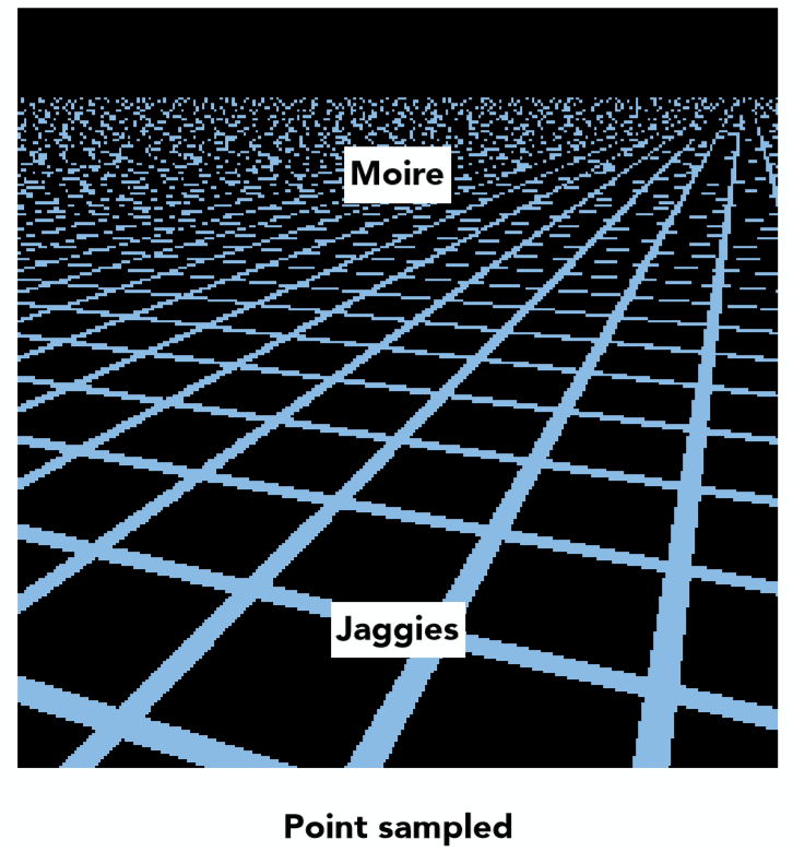
Take nearest sampling as an example, the color of the sample pixel is the color of the nearest texel, and all the rest corresponding texels are ignored. This could cause serious aliasing.
As discussed in previous tasks, bilinear sampling has been proven effective in reducing aliasing. However, averaging the color of all corresponding texels is costly, as the corresponding texel number grows exponentially with the level of minification. Such difficulties are the motivation of mipmaps.
Mipmaps and Level Sampling
Overview
The idea of mipmap is to store a series of downsampled textures, the downsampling process has averaged color ahead of time. When the rasterizer is doing texture mapping, it can choose the finest mipmap level in which each texel has a similar size to the sample pixel. This way, the rasterizer can avoid the expensive averaging process and still get a smooth color transition.
The key considerations of mipmaps is how to choose the mipmap level. Once mipmap level is chosen, normal sampling process, including nearest sampling and bilinear sampling, can be applied to the chosen mipmap.
Mipmap Level Selection
According to the lecture, mipmap level selection can be done in several approaches:
- Fixed mipmap level: The mipmap level is chosen ahead of time, and the same level is used for all sample pixels. This is the simplest approach, and very similar to sampling without mipmaps.
- Nearest level: Based on the size of the sample pixel, the level with the closest texel size is chosen.
- Nearest level with interpolation: Select two closest levels and sample them, this will result in two selected colors. Then, the final color is interpolated between the two colors based on the size of the sample pixel.
Calculation of Closest Mipmap Level
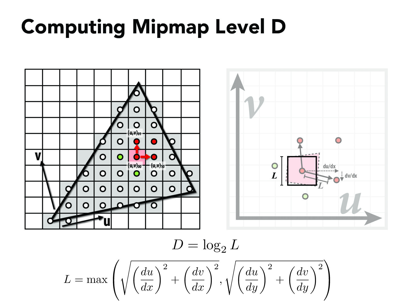
Assuming all mipmaps have the same aspect ratio as the original texture and the sample space, mipmap level could be calculated by inspecting the distance zoom ratio between two sample pixels and their corresponding texels. Let \(L\) be the zoom level of distance, then the mipmap level \(D\) can be calculated as:
As each mipmap level is downsampled by a factor of 2.
However, mipmaps do not always have the same aspect ratio as the original texture and the sample space. In this case, the three nearest pixels of the sample pixel is selected, distance zoom ratio is calculated based on the sample pixel and the x-direction nearest, and y-direction nearest respectively. The mipmap level is then calculated based on the largest distance zoom ratio, as shown in the course slides.
Sample Combinations
The final color of the sample pixel is the color of the chosen mipmap level's texel. The color of the texel is calculated by normal sampling process, including nearest sampling and bilinear sampling. The mipmap level is chosen via the method discussed above. Together, there are six combinations of sample processes.
When mipmap is sampled by bilinear sampling and the mipmap level is chosen via nearest level interpolation, the combination is called trilinear sampling.
Implementation
The rasterization pipeline
The rasterization pipeline is modified to include the level sampling process. The following flowchart shows the rasterization pipeline with level sampling:
flowchart TB
  A[Rasterization Pipeline:Start]
  B[Preprocess-Already done:
  Triangle vertices coordinate conversion
  Bounding box calculation];
  C[Nearest Point Set Selection:
  Check sample points' position
  Find the sample points' nearest points
  Calculate their texture coordinates];
  D[Level Sampling:
  Implement the sampler];
  E[Filling Frame Buffer];
  A --> B;
  B --> C;
  C -->|SampleParameters| D;
  D -->|Color| E;
As the most part has been implemented in previous tasks, the focus of this task is the implementation of the Nearest point set selection and level sampling.
Nearest Point Set Selection
Given the sample pixel, typically its right next pixel and upper next pixel are included in the nearest point set. However, to avoid the potential risk of selecting pixels outside the sample space, when the sample pixel is on the right edge of the bounding box, the left next pixel is included instead of the right one:
        // find the nearest sample points
        // the x and y coordinates of the nearest sample points
        // in the order of current sample point, x nearest sample point, y nearest sample point
        // consider the edge case
        if (current_x_position == bounding_box_x_max)
        {
          current_nearest_x = Vector3D(current_x_position + 0.5, current_x_position - 0.5, current_x_position + 0.5);
        }
        else
        {
          current_nearest_x = Vector3D(current_x_position + 0.5, current_x_position + 1.5, current_x_position + 0.5);
        }
The same applies to the y direction.
        if (current_y_position == bounding_box_y_max)
        {
          current_nearest_y = Vector3D(current_y_position + 0.5, current_y_position + 0.5, current_y_position - 0.5);
        }
        else
        {
          current_nearest_y = Vector3D(current_y_position + 0.5, current_y_position + 0.5, current_y_position + 1.5);
        }
Then, the Barycentric coordinates of the three points are calculated. The first, second and third weights of the Barycentric coordinates are stored in three 3D vectors, weight_0, weight_1, weight_2 respectively.
        // calcuate the weights of the barycentric coordinates
        weight_0 = (-(current_nearest_x - Vector3D(x1_ss)) * line12_delta_y + (current_nearest_y - Vector3D(y1_ss)) * line12_delta_x)/(-(x0_ss - x1_ss) * line12_delta_y + (y0_ss - y1_ss) * line12_delta_x);
        weight_1 = (-(current_nearest_x - Vector3D(x2_ss)) * line20_delta_y + (current_nearest_y - Vector3D(y2_ss)) * line20_delta_x)/(-(x1_ss - x2_ss) * line20_delta_y + (y1_ss - y2_ss) * line20_delta_x);
        weight_2 = (-(current_nearest_x - Vector3D(x0_ss)) * line01_delta_y + (current_nearest_y - Vector3D(y0_ss)) * line01_delta_x)/(-(x2_ss - x0_ss) * line01_delta_y + (y2_ss - y0_ss) * line01_delta_x);
Next, the weight of the sample point is examined to check if the sample point is inside the triangle. If so, the texture coordinates of the nearest point set are calculated, and a new SampleParams object is created.
        // check if the pixel is inside the triangle
        if (weight_0[0] >= 0. && weight_1[0] >= 0. && weight_2[0] >= 0.)
        {
          // if so, calculate the the uv coordinates of the corresponding texel
          current_uv = Vector2D(u0, v0) * weight_0[0] + Vector2D(u1, v1) * weight_1[0] + Vector2D(u2, v2) * weight_2[0];
          // doesn't matter if dx or dy is negative, as we only need the magnitude
          current_dx_uv = Vector2D(u0, v0) * weight_0[1] + Vector2D(u1, v1) * weight_1[1] + Vector2D(u2, v2) * weight_2[1];
          current_dy_uv = Vector2D(u0, v0) * weight_0[2] + Vector2D(u1, v1) * weight_1[2] + Vector2D(u2, v2) * weight_2[2];

          // create a SampleParams struct
          sp.p_uv = current_uv;
          sp.p_dx_uv = current_dx_uv;
          sp.p_dy_uv = current_dy_uv;
          sp.lsm = lsm;
          sp.psm = psm;

          // call the tex.sample function
          current_color = tex.sample(sp);

          // fill the corresponding buffer
          sample_buffer[current_y_position * width * zoom_coefficient + current_x_position] = current_color;

        }
The SampleParams object is then passed to the level sampling process, which will finish the sample process and return the color of the sample pixel. The final step is to fill the corresponding buffer with the returned color.
Sampler
The sampler requires a continuous mipmap level value to implement nearest level and interpolation sampling. This is done by get_level function.
The calculation process follows the method discussed in the methodology section. Noting that the texture coordinates should be scaled to the texture size.
The calculated level is only valid in the range of the mipmap levels. In the case of texture minification, the calculated level could be negative and need to be clamped to 0. In extreme cases, the calculated level could be larger than the number of mipmap levels and need to be clamped to the largest level.
To avoid calculating the largest level every time, the largest level is stored in the Texture class as a member variable.
struct Texture {
  size_t width;
  size_t height;
  std::vector<MipLevel> mipmap;
  int numSubLevels;

  void init(const vector<unsigned char>& pixels, const size_t& w, const size_t& h) {
    width = w; height = h;

    // A fancy C++11 feature. emplace_back constructs the element in place,
    // and in this case it uses the new {} list constructor syntax.
    mipmap.emplace_back(MipLevel{width, height, pixels});

    generate_mips();

    numSubLevels = (int)(log2f((float)max(width, height)));
  }
}
Combining all these considerations, the get_level function is implemented as follows:
  float Texture::get_level(const SampleParams& sp) {
    // TODO: Task 6: Fill this in.
    // calculate the level of the mipmap to sample from
    float Lx, Ly, L, D;
    Lx = sqrt(pow((sp.p_dx_uv.x - sp.p_uv.x) * width, 2) + pow((sp.p_dx_uv.y - sp.p_uv.y) * height, 2));
    Ly = sqrt(pow((sp.p_dy_uv.x - sp.p_uv.x) * width, 2) + pow((sp.p_dy_uv.y - sp.p_uv.y) * height, 2));
    L = max(Lx, Ly);

    D = log2(L);

    // in texture magnification, many pixels are mapped to one texel, so the level should be 0
    if (D < 0)
    {
      D = 0;
    }

    // in extreme texture minification, one texel is mapped to many pixels, so the level should be the maximum level

    if (D > numSubLevels - 1)
    {
      D = numSubLevels - 1;
    }
    return D;
  }
The rest part of the sampler is straightforward, which uses several if statements to cover all sample combinations.
Always sample at 0 level:
    if (sp.lsm == L_ZERO)
    {
      // sample from mipmap level 0
      if (sp.psm == P_NEAREST)
      {
        return sample_nearest(sp.p_uv, 0);
      }
      else if (sp.psm == P_LINEAR)
      {
        return sample_bilinear(sp.p_uv, 0);
      }
      else
      {
        return Color(1, 0, 1);
      }
    }
Nearest level sampling:
    else if (sp.lsm == L_NEAREST)
    {
      // sample from the nearest mipmap level
      int level = (int)round(get_level(sp));

      if (sp.psm == P_NEAREST)
      {
        return sample_nearest(sp.p_uv, level);
      }
      else if (sp.psm == P_LINEAR)
      {
        return sample_bilinear(sp.p_uv, level);
      }
      else
      {
        return Color(1, 0, 1);
      }
    }
Nearest level with interpolation sampling:
    else if (sp.lsm == L_LINEAR)
    {
      // sample from the two nearest mipmap levels and linearly interpolate
      Color c0, c1, result;
      if (sp.psm == P_NEAREST)
      {
        c0 = sample_nearest(sp.p_uv, floor(get_level(sp)));
        c1 = sample_nearest(sp.p_uv, ceil(get_level(sp)));
      }
      else if (sp.psm == P_LINEAR)
      {
        c0 = sample_bilinear(sp.p_uv, floor(get_level(sp)));
        c1 = sample_bilinear(sp.p_uv, ceil(get_level(sp)));
      }
      else
      {
        result = Color(1, 0, 1);
      }
      result = c0 * (1 - get_level(sp) + floor(get_level(sp))) + c1 * (get_level(sp) - floor(get_level(sp)));
      return result;
    }
c0 and c1 are the colors of the two nearest mipmap levels, and result is the final color of the sample pixel. Two nearest levels are determined by the floor and ceil function.
Results
A carefully selected example is used to demonstrate the effect of level sampling. The original texture is a 3840 * 2160 resolution screenshot of the computer game Atomic Heart.

SVG svg/texmap/test6.svgis modified and stored as docs/test6.svg to apply the texture.
To recode the rasterizing time of SVG, clock function is applied to the draw end. The rasterization time of each sampling combination is recorded.
The following figures show the rasterization option of (level 0 sampling, nearest sampling, sample rate 1) and (level 0 sampling, nearest sampling, sample rate 16). The left figure is the simplest case without any particular sampling technique, and the other one is used as an example of no aliasing.


While the left one is aliased, it only takes 0.013008 seconds to rasterize. The right one is much smoother, but it takes 0.07369 seconds to rasterize. The rasterization time is increased by 5.66 times.
The following figures shows the effect of level sampling. The left figure has option (nearest level sampling, nearest sampling, sample rate 1) and the right one has option (nearest level with interpolation sampling, nearest sampling, sample rate 1). The rasterization time of the two is 0.007655 and 0.017561 seconds respectively.


With nearest-level sampling, as the mipmap texture size is reduced, the rasterization time is even less than the original texture. While nearest-level sampling removed aliasing, because the texture level does not match precisely with the sample pixel's level, the text is blurred. By contrast, nearest level with interpolation sampling has a smoother result, but the rasterization time is increased by 2.3 times, which achieves a balance between the quality and the speed.
If level sampling technique is combined with bilinear sampling, the result is even better. The following figures show the comparison of trilinear sampling(left) and supersampling with sample rate 16(right).

The rasterization time of the two is 0.031648 and 0.07369 seconds respectively. The trilinear takes only half of the time of super sampling, while the result is similar.
Conclusion
Level sampling is introduced to solve the aliasing problem in texture magnification and minification without the need for expensive supersampling.
Nearest-level sampling is one simple approach, because of the minification of the texture, the rasterization time is even less than the original texture, as well as the memory consumption. It can remove aliasing, but result might be blurred as the texture level does not match precisely with the sample pixel's level.
Nearest level with interpolation sampling has a smoother result, but loading two nearest levels and linearly interpolating color requires more time and memory. Based on the test, it achieves a balance between the quality and the speed.
Level sampling techniques can be combined with bilinear sampling to achieve even better results. For example, in our test, trilinear sampling achieves the best result along all sample combinations except for supersampling. While the rasterization time is also the second longest, it is trivial when compared to the time of supersampling, and the memory consumption is close to nearest level with interpolation sampling.
Ended: Homework1
Homework2 ↵
Homework2: Meshedit Overview
Overview
From this homework, we learned and practiced the following concepts: - Halfedge Mesh: We implemented a halfedge mesh data structure and various operations on it. - MeshEdit: We implemented various mesh editing operations, such as edge flip, edge split, and vertex split. - Bezier Curve and Patch: We implemented the de Casteljau's algorithm to evaluate points on a Bézier curve and patch.
Besides key concepts, throughout the homework, we also learned about the following: - Debugging large codebase: We learned how to debug a large, unfamiliar codebase. - Code organization: We learned how to make code more readable and maintainable.
Updates to the website
We implemented the following updates to the website:
- Added .csv table support
- Added print webpage button for each page
Note for PDF
Some features of the website, such as picture lightbox, may not be available in the PDF version. We recommend reading the website directly for the best experience.
Section1 ↵
Part 1: Bezier Curves with 1D de Casteljau Subdivision
Methodology
de Casteljau's algorithm is a recursive algorithm that can be used to evaluate a Bezier curve. A Bezier curve is defined by a set of control points, and the curve itself is a linear combination of these control points. Assuming \(t\) to be the proportion of the curve that has been traversed, this algorithm can find the corresponding point's position \(B(t)\) from the curve.
The de Casteljau's algorithm can be described as follows:
-
Given a set of control points \(P_0, P_1, \dots, P_n\), an empty intermediate point set \(Q\) and a parameter \(t\). Set \(Q = P\).
-
Check if the length of \(Q\) is 1. If so, return the only point in \(Q\).
-
Otherwise, for each pair of points \(Q_i, Q_{i+1}\) in \(Q\), calculate the point by linear interpolating:
- Set \(Q = Q'\) and repeat from step 2.
Among each loop, the number of points in \(Q\) will decrease by 1, and the last point in \(Q\) will be the point on the Bezier curve. To draw a Bezier curve, we can progressively evaluate the curve at different \(t\) values and connect the points together.
Implementation
In this task, we are required to implement the interpolate function of de Casteljau's algorithm. The function takes a list of intermediate points and a parameter t, and returns the new intermediate points after interpolation.
The implementation idea is simple: for each pair of points in the input points vector, calculate the intermediate point and store it in the result vector:
  std::vector<Vector2D> BezierCurve::evaluateStep(std::vector<Vector2D> const &points)
  {
    // TODO Part 1.
    // Implement by Ruhao Tian starts here

    // Create a vector iterator
    std::vector<Vector2D>::const_iterator it = points.begin();

    // Create a empty vector to store the result
    std::vector<Vector2D> result;

    // Loop through the points and calculate the intermediate points
    // iterater should stop at the second last point
    while (it != points.end() - 1)
    {
      // Calculate the intermediate point
      Vector2D intermediate = (1 - t) * (*it) + t * (*(it + 1));
      // Add the intermediate point to the result vector
      result.push_back(intermediate);
      // Move the iterator to the next point
      it++;
    }

    return result;
  }
Results
A 6-point Bezier curve is created to test the implementation:
The figures below show the drawn curve as well as levels of evaluation. The left one is the curve without moving control points, and the right one is the curve with control points manually moved.


Part2: Bezier Surfaces with Separable 1D de Casteljau
Methodology
The main way to use de Casteljau's algorithm on the surface is: First, split the two-dimensional control point matrix into n one-dimensional matrices. Then, apply a method similar to Part 1 to each of these n one-dimensional matrices, obtaining coordinates for n points. Finally, use these n points coordinates for one more calculation to get the target point.
The detailed steps are listed as follows:
-
Given a two-dimensional control point matrix P (n rows and m columns). Split the two-dimensional control point matrix into n rows.
-
Apply the de Casteljau's algorithm separately to these n columns, and iterate m-1 times to obtain n final points. This operation is similar to Part 1, where n control points and parameter \(t\) are used to obtain points on the Bézier curve, except here the parameter is \(u\).
-
Use these n points to perform the same operation(parameter is \(v\)), obtaining a point that lies on the Bézier patch.
Summary: A total of \(n * (m-1) + 1\) iterations are required. There are n columns in total, each column requires m-1 iterations. Finally, the n points are iterated once more.
Implementation
The task requires returning a point that lies on the Bézier surface.
First, evaluates one step of de Casteljau's algorithm using the given points and the scalar parameter t.
  std::vector<Vector3D> BezierPatch::evaluateStep(std::vector<Vector3D> const &points, double t) const
  {
    // TODO Part 2.
    std::vector<Vector3D>newPoints;

    double x,y,z;
    for(int i=0;i<points.size()-1;i++){
      x=points[i].x*t+points[i+1].x*(1-t);
      y=points[i].y*t+points[i+1].y*(1-t);
      z=points[i].z*t+points[i+1].z*(1-t);
      newPoints.emplace_back(x,y,z);
    }
    return newPoints;
  }
Second, fully evaluates de Casteljau's algorithm for a vector of points at scalar parameter t.
  Vector3D BezierPatch::evaluate1D(std::vector<Vector3D> const &points, double t) const
  {
    // TODO Part 2.

    //Below is for iteration. If its size==1, it is the goal point.
    std::vector<Vector3D>operatePoints=points;

    double x,y,z;
    while(operatePoints.size()>1){
      operatePoints=evaluateStep(operatePoints,t);
    }
    return operatePoints.front();
  }
Finally, evaluate the Bezier patch at parameter (u, v)
Vector3D BezierPatch::evaluate(double u, double v) const
  {
    // TODO Part 2.

    //Fully evaluate de Casteljau's algorithm for each row of the
    //two-dimensional control. Result is rowPoints.
    std::vector<Vector3D> rowPoints;
    for(int i=0;i<controlPoints.size();i++){
      rowPoints.push_back(evaluate1D(controlPoints[i],u));
    }

    //Fully evaluate de Casteljau's algorithm for rowPoints
    //Result is patchPoint(the goal)
    Vector3D patchPoint;
    patchPoint=evaluate1D(rowPoints,v);
    return patchPoint;
  }
Results
The figures below show the drawn picture of the teapot.bez

Ended: Section1
Section2 ↵
Part 3: Area-Weighted Vertex Normals
Methodology
Given a vertex on the mesh, the normal vector of the vertex is the average of the normal vectors of all the triangles that share the vertex. Assume \(N_0, N_1, \dots, N_k\) are the normal vectors of the triangles that share the vertex, the normal vector of the vertex is calculated as follows:
where \(A_0, A_1, \dots, A_k\) are the areas of the triangles that share the vertex. The normal vector is normalized to ensure it has a unit length.
Implementation
The general idea is to iterate through all faces and calculate the normal vector and area of each face. In halfedge data structure, each face has a corresponding halfedge, and visiting the next face counter-clockwise is equal to visiting its half edge:
And when current_halfedge == start_halfedge, the iteration is finished.
For each face, the normal vector can be obtained by the provided normal function:
To calculate the area of the face, first, the three vertices of the face are obtained:
      vertex_position[0] = current_halfedge->vertex()->position;
      vertex_position[1] = current_halfedge->next()->vertex()->position;
      vertex_position[2] = current_halfedge->next()->next()->vertex()->position;
Then the area of the face is calculated by the cross product of two edges of the face:
current_face_area = cross(vertex_position[1] - vertex_position[0], vertex_position[2] - vertex_position[0]).norm() / 2;
During the iteration, the normal vector and area of each face are accumulated to an intermediate normal vector, which will be normalized and returned when the iteration is finished:
Putting all the pieces together, the implementation of the normal function is as follows:
  Vector3D Vertex::normal( void ) const
  {
    // TODO Part 3.
    // Returns an approximate unit normal at this vertex, computed by
    // taking the area-weighted average of the normals of neighboring
    // triangles, then normalizing.

    // Implementaion by Ruhao Tian starts here

    // Prepare intermediate variables
    HalfedgeCIter current_halfedge, start_halfedge, next_halfedge;
    Vector3D intermediate_normal,current_face_normal;
    double current_triangle_area;
    Vector3D vertex_position[3];

    // Initialize the normal vector
    intermediate_normal = Vector3D(0, 0, 0);
    current_halfedge = start_halfedge = this->halfedge();

    // Loop through the halfedges of the vertex
    do {
      // for safety, first obtain the next halfedge, although this is not mandatory
      next_halfedge = current_halfedge->twin()->next();

      // obtain the face normal
      current_face_normal = current_halfedge->face()->normal();

      // calculate the area of the triangle
      // first, obtain the three vertices position
      vertex_position[0] = current_halfedge->vertex()->position;
      vertex_position[1] = current_halfedge->next()->vertex()->position;
      vertex_position[2] = current_halfedge->next()->next()->vertex()->position;
      // use the cross product to calculate the area
      current_triangle_area = cross(vertex_position[1] - vertex_position[0], vertex_position[2] - vertex_position[0]).norm() / 2;

      // add the area-weighted normal to the intermediate normal
      intermediate_normal += current_face_normal * current_triangle_area;

      // move to the next halfedge
      current_halfedge = next_halfedge;
    } while (current_halfedge != start_halfedge);

    // normalize the intermediate normal
    intermediate_normal.normalize();
    return intermediate_normal;
  }
Results
The left figure below is the screenshot of dae/teapot.dae without normal vector shading and the right one is the same mesh with normal vector shading enabled. Compared with the left one, figure implemented normal vector clearly has smoother shading.
Image displayed size too small?
Click on the image to activate lightbox mode. In lightbox mode, click on the arrows on the left and right to navigate through images. This brings easy comparison.


Part2: Bezier Surfaces with Separable 1D de Casteljau
Methodology
Get the flip image by modifying the given halfedge and related parameter pointers. Below is an example of modifications made to a halfedge:
As shown in the diagram, we now need to modify the pointers related to the halfedge h.

After modification: 1. The starting point of the halfedge becomes A, and it points to D. 2. The twin() of the halfedge remains unchanged, but it now points to the modified halfedge in the opposite direction. 3. The next() of the halfedge becomes CB. 4. The face which the halfedge points to becomes ABC.
Similar operations will also be performed on vertices, faces, and so on. This includes but is not limited to, the following changes: The half-edge pointed to by A becomes h. The faces change from ABD, BCD to ABC, ACD.
The rest of the operations are very similar, so I won't go into further detail. But you can see any information in code.
Implementation
Before providing my code, I would like to explain the parameters:
- h is the h shown in the diagram.
- th=h->twin()
- h/th_next=h/th->next()
- h/th_pre->next()=h/th
v1,v2,v3,v4 is A,B,C,D
VertexIter v1=h_pre->vertex();
VertexIter v2=h->vertex();
VertexIter v4=th_pre->vertex();
VertexIter v3=th->vertex();
Total solution code:
EdgeIter HalfedgeMesh::flipEdge( EdgeIter e0 )
{
// TODO Part 4.
// This method should flip the given edge and return an iterator to the flipped edge.
//edge is not allowed
if(e0->isBoundary()) return e0;
  HalfedgeIter h=e0->halfedge();
  HalfedgeIter th=h->twin();
  HalfedgeIter h_next=h->next();
  HalfedgeIter th_next=th->next();
  HalfedgeIter h_pre=h_next->next();
  HalfedgeIter th_pre=th_next->next();
  VertexIter v1=h_pre->vertex();
  VertexIter v2=h->vertex();
  VertexIter v4=th_pre->vertex();
  VertexIter v3=th->vertex();
FaceIter f1=h->face();
FaceIter f2=th->face();
//change the halfedge pointer
h->setNeighbors(th_pre,th,v1,h->edge(),f1);
th_pre->setNeighbors(h_next,th_pre->twin(),v4,th_pre->edge(),f1);
h_next->setNeighbors(h,h_next->twin(),v3,h_next->edge(),f1);
th->setNeighbors(h_pre,h,v4,h->edge(),f2);
h_pre->setNeighbors(th_next,h_pre->twin(),v1,h_pre->edge(),f2);
th_next->setNeighbors(th,th_next->twin(),v2,th_next->edge(),f2);
//change the vertex pointer
v1->halfedge()=h;
v2->halfedge()=th_next;
v3->halfedge()=h_next;
v4->halfedge()=th;
//change the face pointer
f1->halfedge()=h;
f2->halfedge()=th;
return e0;
}
Results
The figure below shows the original teapot.

The following image shows the teapot after flipping 4 edges. I have highlighted the modifications with a yellow highlighter.

Debug experience
I used to make a very simple but fatal problem, which I used HalfedgeCIter instead of HalfedgeIter. So, I found the program always occurred crashed. Finally, with the assistance of my partner and the ChatGPT, I noticed and understood the difference between CIter and Iter.
Part 5: Edge Split
Methodology
The method of edge splitting is similar to Part 4, but it will be a bit more complex. This requires us to consider a new vertex and the 6 new halfedges that are created. We adjust their values and pointers to accomplish the edge split. Here is a simple example explaining the adjustment of pointers for the halfedge h and the new vertex E.

for h after modification:
- The starting point of the halfedge remains B, but it points to E now.
- The twin() becomes the EB.
- The next() of the halfedge becomes EA.
- The face that the halfedge points to becomes ABE.
for e after modification:
- Its position is descripted by \((E_x,E_y)=0.5*[(B_x,B_y)+(D_x,D_y)]\)
- It points to ED.
Similar operations will also be performed on vertices, faces, and so on. This includes, but is not limited to, the following changes:
- The half-edge pointed to by A becomes AE
- Now there are four faces (ABE, AED, DEC, BEC)
The rest of the operations are similar.
Implementation
Notations of the implementation are shown in the following figure:

To assist coding, data structures and relevant values before and after the edge split are listed in the following tables.
For the halfedges:
| name | next | twin | vertex | edge | face |
|---|---|---|---|---|---|
| j | k | j_twin | a | ab | f1 |
| k | l | o | b | bc | f1 |
| l | j | l_twin | c | ca | f1 |
| m | n | m_twin | b | bd | f2 |
| n | o | n_twin | d | dc | f2 |
| o | m | k | c | bc | f2 |
| j‘ | x | j_twin | a | ab | f3 |
| k’ | l | o | e | ec(bc) | f1 |
| l‘ | p | l_twin | c | ca | f1 |
| m’ | s | m_twin | b | bd | f4 |
| n‘ | o | n_twin | d | dc | f2 |
| o’ | r | k | c | ec(bc) | f2 |
| p‘ | k | q | a | ae | f1 |
| q’ | j | p | e | ae | f3 |
| r‘ | n | s | e | ed | f2 |
| s’ | y | r | d | ed | f4 |
| x‘ | q | y | b | be | f3 |
| y’ | m | x | e | be | f4 |
Where the new halfedges are marked with single quotes, the same applies to the vertices, edges and faces.
For the vertices:
| name | a | b | c | d | a' | b' | c' | d' | e' |
|---|---|---|---|---|---|---|---|---|---|
| halfedge | j | k/m | o/l | n | p/j | x/m | o/l | s/n | k |
For the edges:
| name | ab | bc | ca | bd | dc | ab' | be' | ea' | ec'(bc) | ca' | bd' | dc' | de' |
|---|---|---|---|---|---|---|---|---|---|---|---|---|---|
| halfedge | j | k/o | l | m | n | j | x/y | q/p | k | l | m | n | r/s |
For the faces:
| name | f1 | f2 | f1' | f2' | f3' | f4' |
|---|---|---|---|---|---|---|
| halfedge | j/k/l | m/n/o | l/p/k | o/r/n | j/x/q | m/s/y |
With help of the above tables, the implementation is simple as follows:
VertexIter HalfedgeMesh::splitEdge( EdgeIter e0 )
  {
    // TODO Part 5.
    // This method should split the given edge and return an iterator to the newly inserted vertex.
    // The halfedge of this vertex should point along the edge that was split, rather than the new edges.
    HalfedgeIter j, k, l, m, n, o, j_new, k_new, l_new, m_new, n_new, o_new, p_new, q_new, r_new, s_new,x_new,y_new;
    k_new = k = e0->halfedge();
    l_new = l = k->next();
    j_new = j = l->next();
    o_new = o = e0->halfedge()->twin();
    m_new = m = o->next();
    n_new = n = m->next();
    p_new = newHalfedge();
    q_new = newHalfedge();
    r_new = newHalfedge();
    s_new = newHalfedge();
    x_new = newHalfedge();
    y_new = newHalfedge();

    VertexIter a, b, c, d, a_new, b_new, c_new, d_new, e_new;
    a_new = a = j->vertex();
    b_new = b = k->vertex();
    c_new = c = l->vertex();
    d_new = d = n->vertex();
    e_new = newVertex();

    EdgeIter ab, bc, ca, bd, dc, ab_new, bc_new_ec, ca_new, bd_new, dc_new, ae_new, be_new, ed_new;
    ab_new = ab = j->edge();
    bc_new_ec = bc = k->edge();
    ca_new = ca = l->edge();
    bd_new = bd = m->edge();
    dc_new = dc = n->edge();
    ae_new = newEdge();
    be_new = newEdge();
    ed_new = newEdge();

    FaceIter f1, f2, f1_new, f2_new, f3_new, f4_new;
    f1_new = f1 = k->face();
    f2_new = f2 = o->face();
    f3_new = newFace();
    f4_new = newFace();

    // Update the halfedges
    j_new->setNeighbors(x_new, j->twin(), a, ab, f3_new);
    k_new->setNeighbors(l,o,e_new,bc,f1);
    l_new->setNeighbors(p_new,l->twin(),c,ca,f1);
    m_new->setNeighbors(s_new,m->twin(),b,bd,f4_new);
    n_new->setNeighbors(o,n->twin(),d,dc,f2);
    o_new->setNeighbors(r_new,k,c,bc,f2);
    p_new->setNeighbors(k,q_new,a,ae_new,f1);
    q_new->setNeighbors(j,p_new,e_new,ae_new,f3_new);
    r_new->setNeighbors(n_new,s_new,e_new,ed_new,f2);
    s_new->setNeighbors(y_new,r_new,d,ed_new,f4_new);
    x_new->setNeighbors(q_new,y_new,b,be_new,f3_new);
    y_new->setNeighbors(m,x_new,e_new,be_new,f4_new);

    // Update the vertices
    a_new->halfedge() = j;
    b_new->halfedge() = m;
    c_new->halfedge() = l;
    d_new->halfedge() = n;
    e_new->halfedge() = k;

    // Update the edges
    ab_new->halfedge() = j;
    be_new->halfedge() = y_new;
    ae_new->halfedge() = q_new;
    bc_new_ec->halfedge() = k;
    ca_new->halfedge() = l;
    bd_new->halfedge() = m;
    dc_new->halfedge() = n;
    ed_new->halfedge() = s_new;

    // Update the faces
    f1_new->halfedge() = k;
    f2_new->halfedge() = o;
    f3_new->halfedge() = j;
    f4_new->halfedge() = m;

    // Update the position of the new vertex
    // The new vertex should be the average of the two original vertices, b and c
    e_new->position = (b->position + c->position) / 2;
    return e_new;
  }
With careful consideration of the pointers and values, the implementation is one-shot correct and has undergone no debugging process.
Results
The figure below is the original teapot.

After some edge splits:

After a combination of both edge splits and edge flips:

Part 6: Loop Subdivision for Mesh Upsampling
Methodology
Loop subdivision is a mesh upsampling technique for triangle meshes. It is a simple and efficient way to increase the number of triangles in a mesh. The algorithm involves two main steps: triangle subdivision and vertex position update.
Triangle Subdivision
The subdivision of a triangle is done by adding a new vertex at the center of each edge and connecting the new vertices to form 4 new triangles.
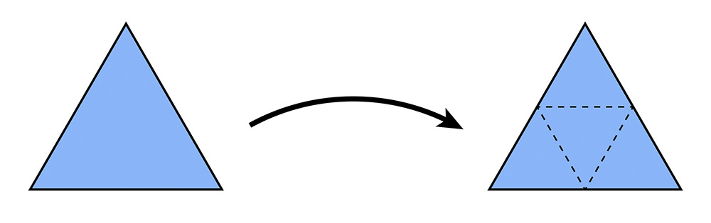
Triangle subdivision can be decomposed into two steps:
- Split all edges of the mesh
- For the new edges, flip the one that connects both new and old vertices
Vertex Position Update
The position of vertices is determined by the surrounding vertices.
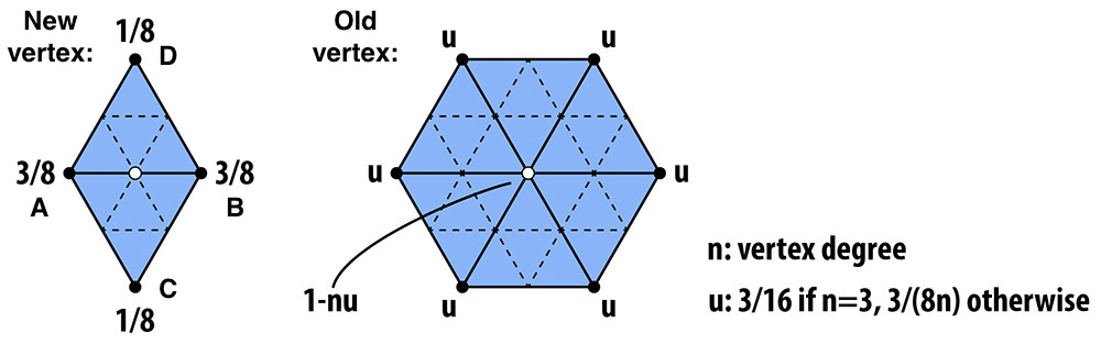
For a new vertex splitting edge \(AB\), the new position is calculated as:
where \(C\) and \(D\) are the vertices of the adjacent triangles to the edge \(AB\).
For an existing vertex, the new position is updated as:
where \(P\) is the original position of the vertex, \(P_i\) is the position of the \(i^{th}\) vertex connected to \(P\), and \(n\) is degree of \(P\). \(u\) is a constant that depends on \(n\), as described in the figure.
Implementation
Subdivision Overview
The recommended steps provided by the course website are followed to implement the Loop subdivision algorithm, as illustrated below:
flowchart TB
  A[Compute new positions for all the vertices in the input mesh]
  B[Compute the updated vertex positions associated with edges];
  C[Split every edge in the mesh];
  D[Flip any new edge that connects an old and new vertex];
  E[Copy the new vertex positions into final Vertex::position];
  A --> B;
  B --> C;
  C --> D;
  D --> E;
Each step is explained in detail in the following sections.
Compute Existing Vertex Positions
Given a vertex in the mesh, the calculation of its updated position involves obtaining all the surrounding vertices and computing the new position based on the degree of the vertex.
To iterate over all connected vertices, halfedge iterator current_halfedge and start_halfedge are used to control the traversal. The degree n is incremented for each visited vertex, and the position of the vertex is added to the sum new_position.
      // initialize the new position
      new_position = Vector3D(0, 0, 0);
      current_halfedge = start_halfedge = v->halfedge();
      n = 0;

      // loop through the halfedges of the vertex
      do
      {
        // add the position of the nearby vertex to the new position
        new_position += current_halfedge->next()->vertex()->position;
        n++;
        // move to the next halfedge
        current_halfedge = current_halfedge->twin()->next();

      } while (current_halfedge != start_halfedge);
When all the surrounding vertices are visited, the new position is updated using the formula provided in the methodology section.
      if (n == 3)
      {
        u = 3.0 / 16.0;
      }
      else
      {
        u = 3.0 / (8.0 * n);
      }
      // calculate the new position
      new_position = (1 - n * u) * v->position + u * new_position;
The above process is repeated for all vertices in the mesh to obtain the updated positions.
Compute New Vertex Positions
A new vertex is added at the midpoint of each edge in the mesh. The new position is calculated using the positions of the two vertices connected by the edge and the positions of the vertices of the adjacent triangles.
First, the four vertices are obtained by halfedge traversal.
      // locate the four surrounding vertices
      VertexIter a = e->halfedge()->vertex();
      VertexIter b = e->halfedge()->twin()->vertex();
      VertexIter c = e->halfedge()->twin()->next()->next()->vertex();
      VertexIter d = e->halfedge()->next()->next()->vertex();
Then, the new position is calculated using the formula provided in the methodology section.
      // calculate the new position for the new vertices
      e->newPosition = 3.0 / 8.0 * (a->position + b->position) + 1.0 / 8.0 * (c->position + d->position);
This step is repeated for all edges in the mesh to obtain the new vertex positions.
Split Edges
In loop subdivision, every edge in the mesh is split once and only once. To prevent repeated splitting, status of each edge need to be tracked. The starter code provides an `Edge::isNew`` flag to indicate whether the edge is new or not.
However, there are multiple definitions of new and old edges in this problem.
- Logical New Edge: An edge that is created during the subdivision process. It is not present in the original mesh. When an old edge is split into two parts, these parts are treated as old edges.
- Chronological New Edge: The edges formed after splitting an old edge are treated as new edges.
For this subsection, both definitions are feasible. However, for the whole problem, only the logical new edge is practical. This will be discussed in the next section.
As logical new edge definition cannot decide whether an edge has been split or not, alternative method is used to track the status of each edge. For a newly split edge, it must connect one new vertex and one old vertex. This way, the edge split can be completed within a single iteration of the mesh edges.
First, all the current edges and vertices are marked as old ones:
    // now every edge in the mesh is old edge
    // set the isNew flag to false for every edge
    for (EdgeIter e = mesh.edgesBegin(); e != mesh.edgesEnd(); e++)
    {
      e->isNew = false;
    }

    // now every vertex in the mesh is old vertex
    // set the isNew flag to false for every vertex
    for (VertexIter v = mesh.verticesBegin(); v != mesh.verticesEnd(); v++)
    {
      v->isNew = false;
    }
Then the iteration begins. For specific edges, check if it is a chronological new edge:
After the edge is split, the chronologically new edges are marked as logically new and old edges:
      // split the edge
      Vector3D new_position = e->newPosition;
      VertexIter new_vertex = mesh.splitEdge(e);
      // set the isNew flag to true for the new edges
      // the original edge, which is now split into two edges, is regarded as a old edge
      HalfedgeIter current_halfedge = new_vertex->halfedge();
      current_halfedge->edge()->isNew = false; // one of the original edges
      current_halfedge = current_halfedge->twin()->next();
      current_halfedge->edge()->isNew = true; // one new edge
      current_halfedge = current_halfedge->twin()->next();
      current_halfedge->edge()->isNew = false; // one of the original edges
      current_halfedge = current_halfedge->twin()->next();
      current_halfedge->edge()->isNew = true; // one new edge
The last step is to process the new vertex. Besides setting it as a new vertex, we immediately assign its newPosition. This is because the edge containing its new position might be flipped in the next section and the pointer to it could be lost.
      // set the isNew flag to true for the new vertex
      new_vertex->isNew = true;
      // set the new position for the new vertex immediately
      // because the edge containing the new vertex might be flipped, and the new position will be lost
      new_vertex->newPosition = new_position;
Flip New Edges
The edges that required flipping are the ones that:
- Is logically new: This is why the logical new edge definition is used. Chronologically new edges are not necessarily flipped, like the ones that are two parts of a split edge.
- Connects an old vertex and a new vertex: As mentioned in the methodology section.
The corresponding code is:
      // check if the edge is a new edge
      if (!e->isNew)
      {
        continue;
      }

      // check if the edge connects an old and new vertex
      if (e->halfedge()->vertex()->isNew==e->halfedge()->next()->vertex()->isNew)
      {
        continue;
      }
      else
      {
        // flip the edge
        mesh.flipEdge(e);
      }
Copy New Vertex Positions
Because both the mesh's original vertices and the ones created by splitting edges have their 'newPosition' set, the final step is to copy the new positions to the original positions.
    // 5. Copy the new vertex positions into final Vertex::position.
    // iterate through all vertices
    for (VertexIter v = mesh.verticesBegin(); v != mesh.verticesEnd(); v++)
    {
      // update the position of the old vertex
      v->position = v->newPosition;
    }
Results
The following images are the upsampling result of dae/torus/input.dae with level 0,1,2, and 3 loop subdivision. The mesh is clearly smoother as the level increases.


One problem is that the sharp edges are smoothed out. Inspecting loop subdivision from a qualitative perspective, the new position of a vertex is determined by its surrounding vertices. This means if a vertex is distant from its neighbors, its distinct position will be averaged out. So to preserve sharp edges, we need to add more vertex around them to strengthen their influence. The following images are the same mesh but with pre-processed outer faces at upsample level 0 and 2. The outer sharp edges are much better preserved.


The same applies to dae/cube.dae. Considering only the face towards us, corner \(A\) is averaged by its three neighbors during upsampling, while corner \(B\) is averaged by two. If we apply this idea recursively to the triangles created by subdivision, we can see that the influence of corner \(A\) is much stronger than corner \(B\). This is why corner \(A\) is much smoother than corner \(B\) in the upsampled mesh.

This provides a hint to solve the asymmetric problem. We need to ensure the structure of neighboring vertices of the corners is symmetric. A simple pre-processing is used in the following figures. The asymmetry is removed after loop subdivision.


Ended: Section2
Ended: Homework2
Homework3 ↵
Homework3: Pathtracer Overview
Overview
In this homework, we implemented a pathtracer that simulates the global illumination of a scene. The pathtracer is capable of simulating the following effects:
- Direct illumination
- Indirect illumination
- BVH acceleration
- Importance sampling
- Russian roulette
Note for PDF
Some features of the website, such as picture lightbox, may not be available in the PDF version. We recommend reading the website directly for the best experience.
Part1: Ray Generation and Scene Intersection
Overview: The ray generation and intersection pipeline
In this part, we implemented the ray generation and intersection pipeline for the Pathtracer. The pipeline consists of the following steps:
flowchart TB
  A[Pixel Sample Generation];
  B[Camera Ray Generation];
  C[Ray-Triangle Intersection];
  D[Ray-Sphere Intersection];
  A --> B;
  B --> C;
  B --> D;
The above sections will be explained in detail in the following sections.
Pixel Sample Generation
Methodology
In the Pathtracer, each pixel of the image is sampled ns_aa times. The input pixel coordinates lie in the unnormalized image space, i.e., the range of the coordinates is from 0 to width and 0 to height.

Each sample process consists of the following steps:
- Generate a random sample point in the pixel space.
- Normalize the sample point to the camera space.
- Generate a ray from the camera origin to the sample point.
- Obtain the returned color and add it to the pixel color.
Implementation
The grid sampler provided in the starter code is used to generate the sample points:
As the width and height of the camera space are 1, the sample point is normalized by dividing the sample point by the width and height of the sample buffer:
      xsample_normalized = ((double)x + sample.x) / sampleBuffer.w;
      ysample_normalized = ((double)y + sample.y) / sampleBuffer.h;
Finally, the ray is generated from the camera origin to the sample point, and the returned color is added to the pixel color:
      // generate a random ray
      r = camera->generate_ray(xsample_normalized, ysample_normalized);
      // trace the ray
      L_out += est_radiance_global_illumination(r);
This process is repeated for ns_aa times to obtain the final pixel color. The result is averaged and assigned to the pixel buffer.
Camera Ray Generation
Methodology
The given pixel position is in the normalized image space. After obtaining its position in the camera space, the ray direction in the camera space is determined. To generate the ray, this direction is transformed to the world space.

Transforming pixel position from the normalized image space to the camera space involves translating the pixel position to the camera space and scaling it by the camera width and height. The translation matrix is given by:
The scaling matrix is given by:
The ray direction in the camera space is the vector from the camera position to the sensor position. The sensor position is obtained by changing the third component of the pixel position to -1.
The camera-to-world matrix the given and does not need to be computed.
Implementation
First, the translation matrix move_to_center and scaling matrix scale_to_sensor are defined:
  // step 1: transform the input image coordinate to the virtual sensor plane coordinate
  // move the input image coordinate to the center of the image plane
  Matrix3x3 move_to_center = Matrix3x3(1, 0, -0.5, 0, 1, -0.5, 0, 0, 1);
  // scale the input image coordinate to the sensor plane coordinate
  // the virtual sensor plane is 1 unit away from the camera
  Matrix3x3 scale_to_sensor = Matrix3x3(2 * tan(radians(hFov / 2)), 0, 0, 0, 2 * tan(radians(vFov / 2)), 0, 0, 0, 1);
The pixel position is transformed to the sensor position by multiplying the translation and scaling matrices:
  // apply the transformation
  Vector3D input_image_position = Vector3D(x, y, 1);
  Vector3D sensor_position = scale_to_sensor * move_to_center * input_image_position;
The ray direction in the camera space is the vector from the camera position to the sensor position:
  // step 2: compute the ray direction in camera space
  // the ray direction is the vector from the camera position to the sensor position
  // in camera space, camera is at the origin
  // simply change the third component of the sensor position to -1
  Vector3D ray_direction_in_camera = {sensor_position.x, sensor_position.y, -1};
Finally, the ray direction is transformed to the world space, and the ray is initialized.
  // step 3: transform the ray direction to world space
  // use the camera-to-world rotation matrix
  Vector3D ray_direction_in_world = c2w * ray_direction_in_camera;

  // normalize the ray direction
  ray_direction_in_world.normalize();

  Ray result = Ray(pos, ray_direction_in_world);
  // initialize the range of the ray
  result.min_t = nClip;
  result.max_t = fClip;

  return  result;
Ray-Triangle Intersection
Methodology
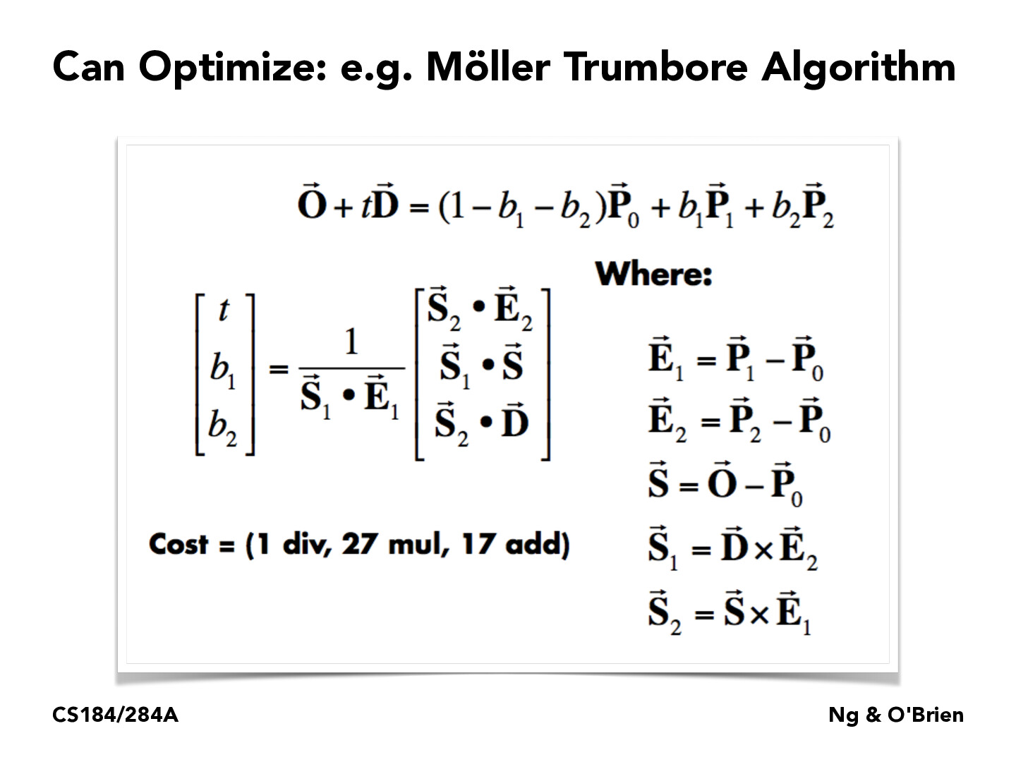
We strictly followed the Moller-Trumbore algorithm to implement the ray-triangle intersection. The algorithm is based on the following steps:
Implementation
First, the Barycentric coordinates of the intersection point and its t value are obtained by the Moller-Trumbore algorithm:
  // Use Moller-Trumbore intersection algorithm
  Vector3D E_1 = p2 - p1;
  Vector3D E_2 = p3 - p1;
  Vector3D S = r.o - p1;
  Vector3D S_1 = cross(r.d, E_2);
  Vector3D S_2 = cross(S, E_1);

  double denominator = dot(S_1, E_1);

  if (denominator == 0) {
    return false;
  }

  double t = dot(S_2, E_2) / denominator;
  double b1 = dot(S_1, S) / denominator;
  double b2 = dot(S_2, r.d) / denominator;
  double b0 = 1 - b1 - b2;
Next, the intersection point is checked:
- If the Barycentric coordinates are inside the triangle.
- If the
tvalue is within the range of the ray.
  // check if t is within the range
  if (t < r.min_t || t > r.max_t) {
    return false;
  }

  // check if b1, b2, and b3 are within the range
  if (b1 < 0 || b1 > 1 || b2 < 0 || b2 > 1 || b0 < 0 || b0 > 1) {
    return false;
  }
If the intersection point is valid, the last step is to update the max_t value of the ray and return true.
Ray-Sphere Intersection
Methodology
For a sphere with center c and radius r, the ray-sphere intersection is calculated by solving the following quadratic equation:
where o is the ray origin, d is the ray direction, and t is the intersection point. The solution to the quadratic equation is given by:
If the part inside the square root is negative, there is no intersection. For this task, we check:
- If there is an intersection.
- If the
tvalue is within the range of the ray.
Implementation
In the test function, whether the ray intersects with the sphere is tested:
bool Sphere::test(const Ray &r, double &t1, double &t2) const {

  // TODO (Part 1.4):
  // Implement ray - sphere intersection test.
  // Return true if there are intersections and writing the
  // smaller of the two intersection times in t1 and the larger in t2.

  // Implementation by Ruhao Tian starts here
  // a t^2 + b t + c = 0
  double a = r.d.norm2();
  double b = 2 * dot(r.d, r.o - o);
  double c = (r.o - o).norm2() - r2;

  // check if there's valid solution
  double delta = b * b - 4 * a * c;
  if (delta < 0) {
    return false;
  }

  // find the two solutions
  double sqrt_delta = sqrt(delta);
  t1 = (-b - sqrt_delta) / (2 * a);
  t2 = (-b + sqrt_delta) / (2 * a);

  return true;

}
The function has_intersection will call test and check further if the intersection point is within the range of the ray:
bool Sphere::has_intersection(const Ray &r) const {

  // TODO (Part 1.4):
  // Implement ray - sphere intersection.
  // Note that you might want to use the the Sphere::test helper here.

  // Implementation by Ruhao Tian starts here
  double t1, t2;
  if (!test(r, t1, t2)) {
    return false;
  }

  // test if t1 is in the valid range
  if (t1 >= r.min_t && t1 <= r.max_t) {
    r.max_t = t1;
    return true;
  }
  else if (t2 >= r.min_t && t2 <= r.max_t) {
    r.max_t = t2;
    return true;
  }

  return false;
}
Results
After implementing the ray generation and intersection pipeline, we obtained the following results:
CBspheres.dae

CBgems.dae

CBcoil.dae

Part 2: Bounding Volume Hierarchy
Constructing the BVH
Methodology
The method I use to construct the BVH (Bounding Volume Hierarchy) is based on splitting at the centroid as the midpoint. The specific choice of the splitting axis is completely random. This ensures that, in the vast majority of cases, the range of leaves will not be too flat.
The specific steps are as follows:
- Select Split Axis: Randomly choose one from the \(x\), \(y\), \(z\) axes as the split axis.
- Calculate Centroid for Selected Axis: Find the position of the centroid along the selected axis
- Sort Pointers According to Coordinates on Selected Axis: Arrange the pointers at this point in order of their corresponding coordinates along the selected axis, from smallest to largest.
- Splitting Nodes: The left subtree contains the first half of the pointers. The right subtree contains the second half of the pointers. Recur this process until the maximum value of nodes is reached.

Implementation
Determine whether the \(max_leaf_size\) has been reached.
if (end - start + 1 <= max_leaf_size){
    node->start = start;
    node->end = end;
    node->l = node->r = NULL;
    return node;
    }
Randomly choose one axis. 0 for x, 1 for y and 2 for z.
Sort pointers according to coordinates on the selected axis.
  std::sort(start, end, [axis](Primitive *a, Primitive *b)
    { return a->get_bbox().centroid()[axis] < b->get_bbox().centroid()[axis]; });
Splitting nodes.
  left_end = start + (end - start) / 2;
  right_start = left_end;
  node->l = construct_bvh(start, left_end, max_leaf_size);
  node->r = construct_bvh(right_start, end, max_leaf_size);
Intersecting the Bounding Box
For most situations: Check the entry and exit times. If the entry time and exit time are in the range between t0 and t1, return True. In addition, the entry time is the maximum of the entry times along each axis, and the exit time is the minimum of the exit times along each axis. Otherwise, return False.

Special Case 1:
If the ray is parallel to one or more axes, let it(or one of them) as axis m. If the value of axis m at the starting position of the ray is within the range of the node, then consider the entry time as negative infinity and the exit time as positive infinity at axis m. Otherwise, return False.
Special Case 2: If the origin of the ray is inside the bounding box, return True.
Special Case 3: If the ray stops in the bounding box, return True.
Implementation
Consider the common situations and the Special Case 1. t[/][0] means the enter time at axis /. t[/][1] means the exit time at axis /. t[0] means axis x. Similarly, t[1] for y and t[2] for z.
  double t[3][2];
  if(r.d.x==0){
    if(r.o.x<min.x||r.o.x>max.x)return false;
    t[0][0]=-99999;
    t[0][1]=999999;
  }
  else{
    t[0][0]=std::min((min.x-r.o.x)/r.d.x,(max.x-r.o.x)/r.d.x);
    t[0][1]=std::max((min.x-r.o.x)/r.d.x,(max.x-r.o.x)/r.d.x);
  }
  if(r.d.y==0){
    if(r.o.y<min.y||r.o.y>max.y)return false;
    t[0][0]=-99999;
    t[0][1]=999999;
  }
  else{
    t[1][0]=std::min((min.y-r.o.y)/r.d.y,(max.y-r.o.y)/r.d.y);
    t[1][1]=std::max((min.y-r.o.y)/r.d.y,(max.y-r.o.y)/r.d.y);
  }
  if(r.d.z==0){
    if(r.o.z<min.z||r.o.z>max.z)return false;
    t[0][0]=-99999;
    t[0][1]=999999;
  }
  else{
    t[2][0]=std::min((min.z-r.o.z)/r.d.z,(max.z-r.o.z)/r.d.z);
    t[2][1]=std::max((min.z-r.o.z)/r.d.z,(max.z-r.o.z)/r.d.z);
  }
  double t_enter = std::max(std::max(t[0][0], t[1][0]), t[2][0]);
  double t_exit = std::min(std::min(t[0][1], t[1][1]), t[2][1]);
Check if the intersection is in the range of t0 and t1
  if (t_exit > t_enter && t_exit > 0)
  {
    if (t_enter > t0 && t_enter < t1)
    {
      t0 = t_enter;
      return true;
    }
  }
  if (r.o.x >= min.x && r.o.x <= max.x && r.o.y >= min.y && r.o.y <= max.y && r.o.z >= min.z && r.o.z <= max.z)
  {
    return true;
  }
  Vector3D end = r.o + r.d * r.max_t;
  if (end.x >= min.x && end.x <= max.x && end.y >= min.y && end.y <= max.y && end.z >= min.z && end.z <= max.z)
  {
    return true;
  }
Intersecting the BVH
Methodology
The core idea is as follows: If it is not a leaf node, recursively check the left and right child nodes. If it is a leaf node, use the function generated in the previous step to check for intersection.
Implementation
BVHAccel:has_intersection
If it is a leaf node.
'''cpp if (node->isLeaf()){ // check if the ray intersects with a bounding box of the node if (!node->bb.intersect(ray, t0, t1))return false; // has intersection, check all primitives in the node for (auto p = node->start; p != node->end; p++){ total_isects++; if ((*p)->has_intersection(ray))return true; } return false; }
If it is not a leaf node, recursively check the left and right child nodes.

```cpp
  bool left_result, right_result;
  left_result = has_intersection(ray, node->l);
  right_result = has_intersection(ray, node->r);
BVHAccel:intersect
This is quite similar to the approach discussed earlier, so I will provide the code directly. More detailed explanations are provided in the comments.
      double t0 = ray.min_t, t1 = ray.max_t;

      // check if current node is leaf node
      if (node->isLeaf())
      {
        // check if the ray intersects with bounding box of the node
        if (!node->bb.intersect(ray, t0, t1))
          return false;

        // has intersection, check all primitives in the node
        bool has_isect = false;
        for (auto p = node->start; p != node->end; p++)
        {
          total_isects++;
          if ((*p)->has_intersection(ray))
          {
            has_isect = true;

            // check the t value of the intersection
            Intersection temp_isect;
            (*p)->intersect(ray, &temp_isect);

            if (temp_isect.t < i->t)
            {
              i->t = temp_isect.t;
              i->primitive = temp_isect.primitive;
              i->n = temp_isect.n;
              i->bsdf = temp_isect.bsdf;
            }
          }
        }
        return has_isect;
      }

      // if current node is not leaf node
      // check if the ray intersects with bounding box of the node
      if (!node->bb.intersect(ray, t0, t1))
        return false;

      // has intersection, check left and right child
      bool left_result, right_result;
      left_result = intersect(ray, i, node->l);
      right_result = intersect(ray, i, node->r);
      // NEVER use 'return intersect(ray, i, node->l) || intersect(ray, i, node->r);'
      // because the right child might not be checked if the left child has intersection
      return left_result || right_result;
Result
Images with normal shading for a few large .dae files that I can only render with BVH acceleration.


I will compare running the following code with and without building the BVH:
Without BVH:
It costs about 13s.
With BVH:

It costs less than 1s.
For the other images:
beast.dae
without BVH

with BVH

beetle.dae
without BVH

with BVH

Summary: Using BVH can be nearly a thousand times faster compared to not using it. For example, rendering beast.dae without BVH takes 3 minutes, while using BVH takes less than half a second. The reason for this is that this structure reduces the number of intersection tests needed to find the intersection between a ray and an object in the scene.
Part3: Direct Illumination
Overview
Global illumination radiance from direct illumination is estimated in this part. The direct illumination consists of zero-bounce and one-bounce light transport, and the latter could be estimated by uniformly sampling the hemisphere or importance sampling the BRDF. The structure of the pipeline is as follows:
flowchart TB
    A[Direct Illumination of Single Ray];
    B[Zero-Bounce Light Transport];
    C[One-Bounce Light Transport];
    D[Uniform Sampling];
    E[Importance Sampling];
    A --> B;
    A --> C;
    C --> D;
    C --> E;
The above sections will be explained in detail in the following sections.
Zero-Bounce Illumination
Methodology
Zero-bounce illumination of a single ray is estimated by adding the emitted radiance from the light sources to the pixel color. The emitted radiance here only considers the light sources and does not consider the indirect illumination from the scene. The rendering equation for zero-bounce illumination is given by:
where \(L_o(p, \omega_o)\) is the radiance leaving the point \(p\) in the direction \(\omega_o\), and \(L_e(p, \omega_o)\) is the emitted radiance from the light sources.
Implementation
In the starter code, the emitted radiance from the intersected light source of the ray is encapsulated in BSDF::get_emission(). The emitted radiance is added to the pixel color and returned:
    // obtain the emission color of the intersection
    Vector3D L_out = isect.bsdf->get_emission();

    return L_out;
Uniform Hemisphere Sampling
Methodology
In physical-based rendering, the reflected radiance from the surface is calculated by integrating the product of the BRDF and the incident radiance over the hemisphere:
where \(L_o(p, \omega_o)\) is the radiance leaving the point \(p\) in the direction \(\omega_o\), \(f(p, \omega_i, \omega_o)\) is the BRDF, \(L_i(p, \omega_i)\) is the incident radiance from the direction \(\omega_i\), and \(\theta_i\) is the angle between the normal and the incident direction.
The integral is approximated by sampling the hemisphere uniformly and averaging the results using Monte Carlo integration:
where \(N\) is the number of samples. For uniform sampling, the possibility function is given by:
The incident radiance can be obtained by zero-bounce illumination, and \(\cos(\theta_i)\) is the dot product between the normal and the incident direction.
The uniform hemisphere sampling calculates \(L_o(p, \omega_o)\) by sampling the hemisphere uniformly and averaging to produce the final result.
Implementation
First, a random direction is sampled in the hemisphere space, and its corresponding vector in world space is also prepared to calculate \(\cos(\theta_i)\):
      // sample a random direction in the hemisphere
      wi_sample_o = hemisphereSampler->get_sample();

      // transform the sample to world space
      wi_sample_w = o2w * wi_sample_o;
      wi_sample_w.normalize();
      // find cos_theta, which is the dot product of the sample direction and the normal
      cos_theta = dot(wi_sample_w, isect.n) / wi_sample_o.norm() / isect.n.norm();
Then a sample ray is generated in the direction of the sampled vector, and the incident radiance is calculated by zero-bounce illumination if the ray intersects with the scene:
      // find the light coming from the sample direction
      // first construct a ray from the hit point to the sample direction
      ray = Ray(hit_p, wi_sample_w);
      ray.min_t = EPS_F;
      Intersection sample_isect;

      // then check if the ray intersects with any object
      if (bvh->intersect(ray, &sample_isect))
      {

        // use zero bounce radiance to calculate the light coming from the sample direction
        wi_sample_incoming_light = zero_bounce_radiance(ray, sample_isect);
      }
      else
      {
        // else there's no light coming from the sample direction
        wi_sample_incoming_light = Vector3D(0, 0, 0);
      }
Finally, the partial result is calculated with Monte Carlo integration and added to the pixel color:
      // for uniform sampling, the probability of each sample is 1 / (2 * PI)
      // now put everything together
      L_out += (1.0 / (double)num_samples) * (cos_theta * isect.bsdf->f(w_out, wi_sample_o) * wi_sample_incoming_light * (2 * PI));
This process is repeated for num_samples times, and the final result is returned.
Importance Sampling
Methodology
Unlike uniform sampling, importance sampling only samples in the direction of light sources. The Monte Carlo integration is also implemented. The render equation is the same as the uniform sampling, but the possibility function is different.
Implementation
The importance sampler will iterate through all the light sources in the scene. Each light source is first checked if it is a delta light(point light source), this is because the result of a point light source is deterministic and only needs to be calculated once. The area light sources are sampled based on their area, a num_total_samples is maintained to perform the normalizing step in the Monte Carlo integration.
      // sample the light
      if (light->is_delta_light())
      {
        num_samples = 1;
      }
      else
      {
        num_samples = ns_area_light;
      }
      num_total_samples += num_samples;
For each sample of each light source, the starter code provides the sample_L function to sample as well as calculates the possibility function.
      // sample the light
      for (int i = 0; i < num_samples; i++)
      {
        wi_sample_incoming_light = light->sample_L(hit_p, &wi_sample_w, &dist_to_light, &pdf);
Again, a ray is generated in the sample direction. However, in importance sampling it is checked that the ray does not hit anything until it reaches the light source.
        // generate a ray from the hit point to the light, check if it hit anything
        ray = Ray(hit_p, wi_sample_w);
        ray.min_t = EPS_F;
        ray.max_t = dist_to_light - EPS_F; // don't forget to subtract EPS_F to avoid self-intersection

        if (bvh->has_intersection(ray))
        {
          continue;
        }
If the ray does not hit anything, the partial result is calculated the same way as in uniform sampling and added to the pixel color.
        // calculate cos_theta
        cos_theta = dot(wi_sample_w, isect.n) / wi_sample_w.norm() / isect.n.norm();
        // calculate the sample direction in object space
        wi_sample_o = w2o * wi_sample_w;

        // put everything together
        L_out += (cos_theta * isect.bsdf->f(w_out, wi_sample_o) * wi_sample_incoming_light) / pdf;
Finally, the result is normalized by num_total_samples and returned.
One-Bounce Illumination and Direct Illumination
One-Bounce Illumination function calls different sampling methods based on user selection:
  Vector3D PathTracer::one_bounce_radiance(const Ray &r,
                                           const Intersection &isect)
  {
    // TODO: Part 3, Task 3
    // Returns either the direct illumination by hemisphere or importance sampling
    // depending on `direct_hemisphere_sample`

    // Implementation by Ruhao Tian starts here

    if (direct_hemisphere_sample)
    {
      return estimate_direct_lighting_hemisphere(r, isect);
    }
    else
    {
      return estimate_direct_lighting_importance(r, isect);
    }
  }
The direct illumination is estimated by adding the zero-bounce and one-bounce illumination to the pixel color:
    // add direct illumination to L_out
    L_out += zero_bounce_radiance(r, isect);

    // TODO (Part 3): Return the direct illumination.
    // add one bounce radiance to L_out
    L_out += one_bounce_radiance(r, isect);
Results
The following images show the results of the direct illumination with uniform sampling and importance sampling.
CBbunny.dae
Uniform Sampling

Importance Sampling

CBspheres_lambertian.dae
Uniform Sampling

Importance Sampling

From the images, it can be observed that the importance sampling produces a smoother result than the uniform sampling. This is because, given the same amount of samples per pixel and per light source, the importance sampling will concentrate more samples on the light sources, which is more efficient than uniformly sampling the hemisphere. Uniform sampling, on the other hand, will waste samples on the directions that do not contribute to the final result, which is why the result is noisier.
The following images are the results of the importance sampling with 1, 4, 16, and 64 light rays and 1 sample per pixel of the CBspheres_lambertian.dae scene.


According to the images, the result becomes smoother as the number of light rays increases. This is because the more light rays are sampled, the more accurate the result will be. However, the result will also be more noisy if the number of samples per pixel is low. This is why the result is still noisy with 64 light rays and 1 sample per pixel. The result will be smoother if the number of samples per pixel is increased, but it will also be more computationally expensive. Therefore, the number of samples per pixel should be chosen based on the trade-off between the quality of the result and the computational cost.
Part4: Global Illumination
Sampling with Diffuse BSDF
Methodology
Using \(sampler.get_sample(pdf)\), a random sample direction is obtained from the cosine-weighted hemisphere distribution. Next, the obtained sample direction \(wi\) is used as the incoming light direction, and the \(f\) function is called to compute the BSDF evaluation of the diffuse material at \((wo, *wi)\).
Implementation
The function \(f\) is defined in Part 3.
Global Illumination with up to N Bounces of Light
Methodology
The following is the rendering equation.

Simplify:


Solve the equation:

Implementation
at_least_one_bounce_radiance
If \(r.depth == max_ray_depth - 1\), this means the maximum depth has been reached. L_out just needs to add the value of this diffuse reflection, which is the function \(one_bounce_radiance\).
Check if the maximum depth is reached. If true, return the L_out. Otherwise, continue operating the rest of the code.Now, calculate the radiance from extra bounces. First, obtain a ray from the hit point to the sample direction.
Vector3D wi_sample_o, wi_sample_w;
double pdf;
Vector3D wi_sample_incoming_light;
Ray ray;
Intersection isect_light;
// sample the next direction
isect.bsdf->sample_f(w_out, &wi_sample_o, &pdf);
// transform the sample direction to object space
wi_sample_w = o2w * wi_sample_o;
// generate a ray from the hit point to the sample direction
double cos_theta = dot(wi_sample_w, isect.n) / wi_sample_w.norm() / isect.n.
norm();
ray = Ray(hit_p, wi_sample_w);
ray.depth = r.depth + 1;
ray.min_t = EPS_F;
Next, recurse this equation until reaching max_ray_depth(this was checked before).
if (bvh->intersect(ray, &isect_light))
{
// calculate the radiance from the extra bounces
L_out += (isect.bsdf->f(w_out, wi_sample_o) * at_least_one_bounce_radiance (ray, isect_light) * cos_theta / pdf);
}
est_radiance_global_illumination
Just need to accumulate the result each time.
Global Illumination with Russian Roulette
Methodology
Now we have set a probability between 0.3 and 0.4 (implemented as 0.35) as the probability for early termination. Due to the influence of probability, we need to normalize the result. The core idea is shown in the diagram below.

Implementation
We just need to make some small adjustments to the function \(at_least_one_bounce_radiance\). The adjusted code is as follows.
First, set the possibility.
Next, check whether to terminate early. if (bvh->intersect(ray, &isect_light) && coin_flip(possibility)){
//Here, a lot of code has been omitted.
return L_out;
}
At last, normalize. Note that the code below has an additional parameter \(probability\).
L_out += (isect.bsdf->f(w_out, wi_sample_o) * at_least_one_bounce_radiance(ray, isect_light) * cos_theta / pdf) / possibility;
Finally, here is the overall code. This is very similar to the previous section, so you don't need to pay too much attention to these codes.
  if (isAccumBounces || r.depth == max_ray_depth - 1)
    {
      L_out += one_bounce_radiance(r, isect);
    }
// check if the maximum depth is reached
  if (r.depth >= max_ray_depth - 1)
    {
    return L_out;
    }
// if not, calculate the radiance from extra bounces
Vector3D wi_sample_o, wi_sample_w;
double pdf;
Vector3D wi_sample_incoming_light;
Ray ray;
Intersection isect_light;
// sample the next direction
isect.bsdf->sample_f(w_out, &wi_sample_o, &pdf);
// transform the sample direction to object space
wi_sample_w = o2w * wi_sample_o;
// generate a ray from the hit point to the sample direction
double cos_theta = dot(wi_sample_w, isect.n) / wi_sample_w.norm() / isect.n.norm();
ray = Ray(hit_p, wi_sample_w);
ray.depth = r.depth + 1;
ray.min_t = EPS_F;
if (bvh->intersect(ray, &isect_light) && coin_flip(possibility))
{
// calculate the radiance from the extra bounces
L_out += (isect.bsdf->f(w_out, wi_sample_o) * at_least_one_bounce_radiance(ray, isect_light) * cos_theta / pdf) / possibility;
}
return L_out;
Results
Here are some direct and indirect illumination.
Direct


Indirect(only sum m=2,3,4,5)


Compare
We can find that the direct illumination is more smooth and lighter than the indirect one.
Here are the results for rendering the mth bounce of light with max_ray_depth set to 0, 1, 2, 3, 4, and 5, and isAccumBounces=false, for CBbunny.dae
m=0

m=1

m=2

m=3

m=4

m=5

Reason
This is because each time the light reflects off a surface, some of its energy is absorbed or scattered, leading to an overall decrease in brightness with each subsequent bounce. As the number of reflections increases for the second and third bounces of light, the intensity of light diminishes, resulting in the images becoming progressively darker.
The main reason it improves the quality of rendered images is that multiple reflections simulate the paths of real light in the physical world, making the images more closely resemble what we see in reality. This enhances the realism of the images. For example, multiple reflections result in more accurate and realistic shadows, which contribute to a more lifelike appearance.
Here are the results for rendered views with max_ray_depth set to 0, 1, 2, 3, 4, and 5 for CBbunny.dae
m=0

m=1

m=2

m=3

m=4

m=5

Compare
We can find that as m increases, the picture becomes brighter and brighter.
Here are the results for outputing the Russian Roulette rendering with max_ray_depth set to 0, 1, 2, 3, 4, and 100 for CBbunny.dae
m=0

m=1

m=2

m=3

m=4

m=100

The following are rendering pictures of the same scene with different sampling rates.
sample-per-pixel rate=1

sample-per-pixel rate=2

sample-per-pixel rate=4

sample-per-pixel rate=8

sample-per-pixel rate=16

sample-per-pixel rate=64

sample-per-pixel rate=1024

Compare
As the sample-per-pixel rate increases, the image will become smoother and smoother. At the same time, the brightness will also increase slightly.
Part5: Adaptive Sampling
Methodology
The high-level idea of adaptive sampling is to reduce the sampling number of pixels that converge to a certain color quickly and focus on the pixels that take longer to converge. A variable \(I\) is maintained to measure the convergence of the pixel:
where \(\sigma\) is the standard deviation of the pixel color samples, and \(n\) is the number of samples.
\(I\) decreases as the number of samples increases and the standard deviation decreases. When \(I\) is less than a certain threshold, the pixel is considered to have converged, and the sampling process stops. The threshold is given by:
where \(\mu\) is the mean of the pixel color samples, and \(\text{maxTolerance}\) is a user-defined parameter, which is set to 0.05 by default.
Implementation
To calculate convergence, two variables total_illumination and total_illumination_squared are maintained:
where \(x_{k}\) is the illumination of sample \(k\).
For one sample, first, the normal sample process mentioned in Part1 is executed:
        // generate a random sample
        current_sample = gridSampler->get_sample();
        // don't forget to normalize the sample
        xsample_normalized = ((double)x + current_sample.x) / sampleBuffer.w;
        ysample_normalized = ((double)y + current_sample.y) / sampleBuffer.h;
        // generate a random ray
        current_ray = camera->generate_ray(xsample_normalized, ysample_normalized);
        // trace the ray
        current_radiance = est_radiance_global_illumination(current_ray);
        L_out += current_radiance;
After the normal sample process, the illumination of the current sample is added to total_illumination`` andtotal_illumination_squared`:
        current_illumination = current_radiance.illum();
        total_illumination += current_illumination;
        total_illumination_squared += current_illumination * current_illumination;
For more efficient processing, the convergence is tested every samplesPerBatch samples:
        if (i % samplesPerBatch == 0)
        {
          // check convergence of the pixel
          mean = total_illumination / (i + 1);

          deviation = sqrt((total_illumination_squared - (i + 1) * mean * mean) / i);

          I = 1.96 * deviation / sqrt(i + 1);

          if (I < maxTolerance * mean)
          {
            break;
          }
        }
If the pixel color is difficult to converge, it is sampled at most ns_aa time, which is the sample number in normal sampling in Part 1.
After the sample process is finished, total radiance L_out is normalized by the actual sample time i and assigned to the sample buffer:
      // take the average of all the samples
      L_out /= i + 1;
      // update the sample buffer
      sampleBuffer.update_pixel(L_out, x, y);
      sampleCountBuffer[x + y * sampleBuffer.w] = i + 1;
Result
The following figures are two scenes rendered with 2048 samples per pixel, a max ray depth of 5 and 1 sample per light.
CBbunny.dae
Render result

Sample rate image

CBdragon.dae
Render result

Sample rate image

Ended: Homework3
Homework4 ↵
Homework4: Clothsim Overview
Overview
Working in progress...
Note for PDF
Some features of the website, such as picture lightbox, may not be available in the PDF version. We recommend reading the website directly for the best experience.
Part 1: Masses and springs
Results
Note: The blurriness comes from the low resolution of the screenshot. The following images show the result of scene/pinned2.json at default parameters:


Wireframe with specific conditions
Without any shearing constraints


With only shearing constraints


With all constraints


Part 2: Simulation via numerical integration
Note: The units of the following data are all default units.
Changing the spring constant ks
ks=50000

ks=5000

ks=500

Description: All these pictures are taken when the cloth becomes static. As ks increases, the spring becomes more difficult to extend and compress. This will cause the fabric to feel tighter. In the picture, it is obvious that the lowest point in the middle of the fabric has been decreasing, and the wrinkles have also increased. Not only that, the acceleration of the cloth will also increase (in the same posture).
Changing the density
density=150

density=15

density=1.5

Description: All these pictures are taken when the cloth becomes static. The effect of changing this parameter is the same as changing ks (in the case of Part 2, i.e. collisions are not considered). Because density is proportional to gravity, gravity is equal to the change of the spring times ks. Therefore, as the density increases, the center becomes lower and lower, and there are more and more wrinkles. Not only that, the acceleration of the cloth will also increase (in the same posture)
Changing the damping
damping approximately equal to 0.9, time= 10s

damping approximately equal to 0.5, time= 10s

damping approximately equal to 0.1, time= 10s

damping = 0

The following are two images representing arbitrary damping when the cloth is still and does not change.


Description: The three pictures above are images of the cloth running from the initial state for 10 seconds. Obviously, the smaller the damping, the faster the cloth will fall. The two pictures below show that when the object is stationary, changing the damping will have no effect (after all, it is not moving). The special case is that the damping is 0. The cloth will never stop due to energy conservation.
scene/pinned4.json in its final resting state


Part 3: Handling collisions with other objects
Note: The units of the following data are all default units.
scene/sphere.json in its final resting state
ks=50000

ks=5000

ks=500

Description: This is because as the spring constant ks increases, the spring becomes harder to extend (or compress). This results in the fabric appearing tighter. The most noticeable effect is that as ks increases, the lowest point of the fabric rises.
Shaded cloth lying peacefully at rest on the plane

Part4: Handling self-collisions
Implementation
To generate a hash value for each point mass, we partitioned the space according to the instructions. To make the hash value unique, we scale the coordinate in each dimension by a factor that is larger than the maximum partition number of all dimensions. The space is partitioned by \(w * h * t\), where \(t = max(w,h)\), so the multiplication factor is \(t\). The hash value is calculated as follows:
  // compute a unique float identifier
  return box_position.x * t * t + box_position.y * t + box_position.z;
Besides choosing the float identifier, the rest process of handling self-collisions is the same as the instruction.
Results
The following images show the result at default parameters:


Then we tested the simulation with different densities and spring constant.
Note for PDF
The following GIFs may not be displayed correctly in the PDF version. We recommend reading the website directly for the best experience.
Density = 150, ks = 5000 & Density = 1.5, ks = 5000


Density = 15, ks = 50000 & Density = 15, ks = 500


Density = 150, ks = 50000 & Density = 1.5, ks = 500


By varying the density and the spring constant the following effects can be observed:
- Density: When density is particularly high, the cloth looks squished and the space between layers of cloth is very small, compared to the normal setting. When density is very low, the space between layers of cloth is larger, and the cloth looks weaker to bend.
- Spring Constant: When the spring constant is high, the internal force causes the cloth to better maintain its shape, quite similar to the effect of low density. When the spring constant is low, the cloth looks weaker to bend, and the space between layers of cloth is also smaller.
- Total effect: It is noticeable that as long as the multiplier of density and spring constant remains the same, the cloth will have similar behavior. For example, when the density is 150 and the spring constant is 5000, the cloth behaves similarly to when the density is 1.5 and the spring constant is 5000.
Part5: Shaders
Task 1: Shader program overview
Shader programs execute on the GPU, run in parallel, and are written in GLSL in this assignment. These programs cover several parts of the graphic pipeline. In this assignment, two types of shaders are used: vertex and fragment shaders. The vertex shader is responsible for transforming the vertices of the object, while the fragment shader is responsible for coloring the pixels of the object.
The vertex shader takes the vertex position, normal, and texture coordinates as input and transforms the vertex position to the screen space. It may also change the normal and texture coordinates to achieve different effects, such as bump mapping. The processed information will be passed to the fragment shader for further processing.
The fragment shader takes the interpolated vertex position, normal, and texture coordinates as input and colors the pixel based on the lighting model and texture mapping. It will be automatically linked to the corresponding vertex shader program if there is one. Together, these two shaders form a shader program that renders objects will different materials and lighting effects.
This flowchart shows the general process of the shader program:
flowchart TB
  A[Application];
  B[Vertex Shader];
  C[Fragment Shader];
  D[Screen Output];
  A -->|Vertex Data| B;
  B -->|Intepolated Data| C;
  C -->|Pixel Color| D;
Task 2: Bling Phong Shading
Methodology
In this part, we implement the Bling Phong shading model in the fragment shader. The Bling Phong shading model consists of three components: ambient, diffuse, and specular.
The ambient component is the light that is reflected by the object from the environment. Bling-Phong shading assumes that the ambient light is constant for each part of the object. The ambient component is calculated by multiplying the ambient coefficient, i.e., how much ambient light is reflected, with the ambient light intensity:
The diffuse component is the diffuse reflection of the object. It is equal to the total irradiance arriving at the surface. Given the radiosity \(I\) of the light source at unit distance, the radiosity of the light source at distance \(r\) is \(I/r^2\). However, according to Lambert's cosine law, the irradiance is proportional to the cosine of the angle between the light source and the normal of the object. Therefore, the diffuse component is calculated as follows:
The specular component is the specular reflection of the object. Specular reflection can only be observed within a certain range of angles. In Bling-Phong shading, a half-vector is used to calculate the specular reflection. The half-vector is the vector that bisects the angle between the light source direction \(\vec{l}\) and the eye direction \(\vec{v}\). The angle between the half-vector and the normal vector \(\vec{n}\) is used to calculate the degradation of the specular reflection:
Where \(p\) is the shininess coefficient. The specular component is calculated as follows:
By adjusting the ambient, diffuse, and specular coefficients, different materials can be simulated.
Implementation
In our implementation, we manually choose a set of Bling-Phong shading parameters as follows:
  // define ka, kd, ks, la, and p
  float ka = 0.1; // Ambient reflection coefficient
  float kd = 0.8; // Diffuse reflection coefficient
  float ks = 0.5; // Specular reflection coefficient
  vec3 la = vec3(1.0, 1.0, 1.0); // Ambient light intensity
  float p = 32.0; // Shininess
First, the output is initialized as a zero vector and the ambient, diffuse and specular component is added, respectively:
  out_color.xyz = vec3(0.0, 0.0, 0.0);

  // ambient reflection
  out_color.xyz += ka * la;

  // diffuse reflection
  float r = length(u_light_pos - v_position.xyz);
  vec3 l = normalize(u_light_pos - v_position.xyz);
  vec3 n = normalize(v_normal.xyz);
  out_color.xyz += kd * u_light_intensity / (r * r) * max(dot(n, l), 0.0);

  // specular reflection
  vec3 v = normalize(u_cam_pos - v_position.xyz);
  vec3 h = normalize(l + v);
  out_color.xyz += ks * u_light_intensity / (r * r) * pow(max(dot(n, h), 0.0), p);

  out_color.a = 1;
Results
The following images show the result of Bling Phong shading with ambient only, diffuse only, specular only, and all components combined.
Ambient Only and Diffuse Only


Specular Only and All Components


Task 3: Texture Mapping
In this part, we implement texture mapping in the fragment shader:
The texture is replaced by an image downloaded from Berkeley Reddit:

The following image shows the result of texture mapping:

Task 4: Bump Mapping and Displacement Mapping
Implementation of Bump Mapping
In this section, we implemented Bump Mapping in the fragment shader by sampling a chosen height map.
First, a local space disturbance vector is created by sampling the height map:
  // calculate dU, dV
  float dU = (h(vec2(v_uv.x + 1.0 / u_texture_2_size.x, v_uv.y)) - h(v_uv)) * u_normal_scaling * u_height_scaling;
  float dV = (h(vec2(v_uv.x, v_uv.y + 1.0 / u_texture_2_size.y)) - h(v_uv)) * u_normal_scaling * u_height_scaling;

  // calculate local space normal
  vec3 n0 = vec3(-dU, -dV, 1.0);
Then, a \(TBN\) matrix is created ahead of time to convert local space vectors to object space:
  // calculate local space tangent
  vec3 t = v_tangent.xyz;

  // calculate local space bitangent
  vec3 n = v_normal.xyz;
  vec3 b = cross(n, t);

  // calculate TBN matrix
  mat3 TBN = mat3(t, b, n);
Finally, the normal is transformed from local space to object space:
This normal is then used in the Bling Phong shading model to calculate the final color.
Implementation of Displacement Mapping
Different from Bump Mapping, in displacement mapping the coordinates of the input vector is also modified in the vertex shader:
Where \(h(v_uv)\) is the height map function. The vertex position is moved along the normal direction by the height map value.
Results
A height map from Wikipedia is used in this part:

The following images show the result of bump mapping and displacement mapping:
Bump Mapping with Coarseness 16 and 128


Displacement Mapping with Coarseness 16 and 128


According to the figures, the sphere with bump mapping has a smooth round shape despite the rough surface caused by the height map. Different from bump mapping, the sphere with displacement mapping has a rough surface and the shape is distorted. This is because the vertex position is modified in the vertex shader, which changes the shape of the object.
Coarseness also affects the result of bump mapping and displacement mapping. The results with less coarseness have more concentrated and brighter specular reflections, while the highlights are more diffused with more coarseness.
Task 5: Environment Mapping
Methodology and Implementation
In this part, we simulate mirror reflection by casting a ray from the camera position to the object and then reflecting it to the environment map.
Given the camera position and fragment position, the eye ray direction is calculated as follows:
The reflected ray direction is calculated with the help of object normal:
  // Calculate the reflection direction
  vec3 reflection_dir = reflect(eye_ray_dir, normalize(v_normal.xyz));
Finally, the environmental map is sampled with the same technique in previous tasks:
  // sample the environment map
  out_color = texture(u_texture_cubemap, reflection_dir);

  out_color.a = 1;
Results
The image below shows the result of environment mapping. The object is a sphere with a mirror reflection. The environment map is a skybox with a mountain view.
