Overview
The project contains two parts that experiments with diffusion models. For the first part, I interact with a pretrain diffusion model DeepFloyd IF to perform several types of image generation. For the second part, I build and train my own diffusion model usingtorch.nn.Module with the MNIST dataset.Part A: The Power of Diffusion Models
Setup
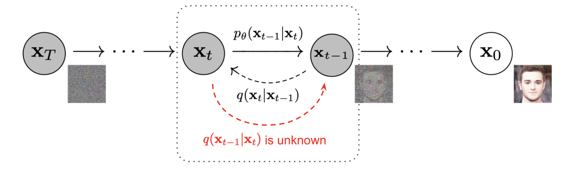
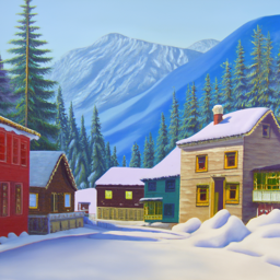
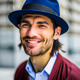
For the whole part, I use the pretrain DeepFloyd IF imported from Hugging Face. The model has two stages. The first one takes in noisy images of size $64\times 64$ and text embeddings to generate a denoised image. The second stage takes in the output of the first stage and generates images of size $256\times 256$.In the forward process, as $t$ increases, the images will get noisier. And the backward process, which is what the denoiser do in stage one of the diffusion model is to estimate the noise in the image.
"a high quality photo" as a default text embeddings if not mentioned specifically.Here's some images generated from the model:

stage 1 |

stage 1 |

stage 1 |
stage 2 |
stage 2 |
stage 2 |

stage 1 |

stage 1 |

stage 1 |
stage 2 |
stage 2 |

stage 2 |
Forward Process
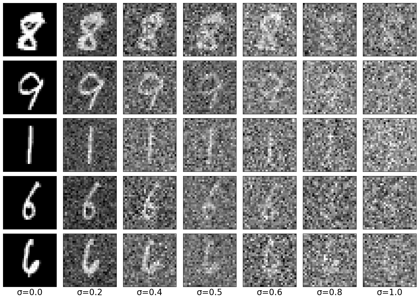
Forward process in diffusion models is to add noise to clean images. The forward process algorithm is defined by: $$q(x_t|x_0)=N(x_t;\sqrt{\bar{\alpha}}x_0, (1-\bar{\alpha}_t)I)$$ is equivalent to: $$x_t=\sqrt{\bar{\alpha}_t}x_0+\sqrt{1-\bar{\alpha}_t}\epsilon \text{ where }\epsilon\sim N(0,1)$$ $x_t$: noisy images$x_0$: clean images
$\epsilon$: noise
$\bar{\alpha}_t$:
alpha_cumprod, determined by the trainer of the model

|

|

|

|
Classical Denoising
Calssically, I use gaussian blur filter to try to get rid of noise. But in this case this classical denoising does not work well.

|

|

|

at t=250 |

at t=500 |

at t=750 |
One-Step Denoising
One step denoising uses the pretrained diffusion model to denoise. The denoiser located atstage_1.unet. This denoiser estimates the noise in the noisy images given the timestep. Then remove the
noise from noisy images can recover the estimate of original images.
|
|
|
|

|

|

|

at t=250 |

at t=500 |

at t=750 |
Iterative Denoising
It's obvious that the Unet denoiser works much better than the Gaussian denoiser. But the result is still blurry as more noise added to the image. To make the performance even better, I implement the iterative denoising. In theory, the diffusion model allows me to iteratively denoising for 1000 timesteps. But to save time, I use a stride of 30 in total timestep of $T=1000$. I generated a list of times stepsstrided_timesteps, with values:
[990, 960, 930, 900, 870, 840, 810, 780, 750, 720, 690, 660, 630, 600, 570, 540, 510, 480, 450, 420, 390, 360, 330, 300, 270, 240, 210, 180, 150, 120, 90, 60, 30, 0]
The denoising algorithm on the
ith step is:
$$x_{t'}=\frac{\sqrt{\bar{\alpha}_{t'}}\beta_t}{1-\bar{\alpha}_t}x_0+\frac{\sqrt{\alpha_t}(1-\bar{\alpha}_{t'})}{1-\bar{\alpha}_t}x_t+v_\sigma$$
$t$: time at strided_timesteps[i]$t'$: time at
strided_timesteps[i+1]$x_t$: image at timestep $t$
$x_{t'}$: image at timestep $t'$
$\bar{\alpha}_t$:
alpha_cumprod$\alpha_t$: $\frac{\bar{\alpha}_t}{\bar{\alpha}_{t'}}$
$\beta_t$: $1-\alpha_t$
$x_0$: the current estimate of clean image as in the one-step denoising
$v_\sigma$: random noise

|

|

|

|

|

|

|
In this part, I use
i_start = 10, which correspondence to timestep 690.
|
Campanile |

at t=690 |

|

|

|
Diffusion Model Sampling
By takingi_start = 0, the algorithm would denoise from pure noise and start generate images.

|

|

|

|

|
Classifier-Free Guidance (CFG)
Some images generated in the previous section are not very good. To improve the quality of images, I use a technicque called Classifier-Free Guidance. In this technicque, the algorithm computes both a conditional and an unconditional noise estimate, then the new noise will be: $$\epsilon=\epsilon_u+\gamma(\epsilon_c+\epsilon_u)$$ By taking $\gamma>1$, we get a much higher quality images. For this and later sections, I use text embeddings"" as the unconditional prompt and "a high quality photo" as the conditional prompt.

|

|

|

|

|
The results compare to the previous section is much more vivid and high-contrast.
Image-to-Image Translation
Image-to-image translation takes in a clean image, adds noise to it to a level, and then denoises it. This allows edits to existings images. The more noise it adds, the larger the edit will be.

|

|

|

|

|

|
|

|

|

|

|

|

|

|

|

|

|

|

|

|

|
Editing Hand-Drawn and Web Images
Except for taking in realistic images, the algorithm can also edit hand-drawn and web images.

|

|

|

|

|

|

|

|

|

|

|

|

|

|

|

|

|

|

|

|

|
Inpainting
Given an image and a mask, I can also generate images that only the masked area changes while other area stays the same. In each loop, the new image will be: $$x_t\leftarrow mx_t+(1-m)\text{forward}(x_{orig},t)$$ $x_{orig}$: original image$m$: binary mask

|

|

|

|

|

|

|

|

|

|

|

|
Text-Conditional Image-toimage Translation
In this section, I experiments image editing by changing different text prompt from"a high quality photo".

t=960 |

t=900 |

t=840 |

t=780 |

t=690 |

t=390 |
|

t=960 |

t=900 |

t=840 |

t=780 |

t=690 |

t=390 |
|

t=960 |

t=900 |

t=840 |

t=780 |

t=690 |

t=390 |
|
Visual Anagrams
In this section, I create optical illusion with diffusion models. The model with generate images that look like one thing normally and another thing up side down. To implement this, the estimate noise from the model is modified according to the algorithm: $$\epsilon_1 = \text{UNet}(x_t, t, p_1)$$ $$\epsilon_2 = \text{flip}(\text{UNet}(\text{flip}(x_t), t, p_2))$$ $$\epsilon = (\epsilon_1 + \epsilon_2)/2$$

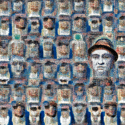
people around a campfire |

an old man |

|

|

|

|
Hybrid Images
In this section, I create another optical illusion that looks like one thing closely and another thing far away. The estimate noise algorithm is modified following the algorithm: $$\epsilon_1 = \text{UNet}(x_t, t, p_1)$$ $$\epsilon_2 = \text{UNet}(x_t, t, p_2)$$ $$\epsilon = f_\text{lowpass}(\epsilon_1) + f_\text{highpass}(\epsilon_2)$$

|

|

|
Part B: Diffusion Models from Scratch
In this part, I will build the denoise Unet from scratch usingtorch.nn. I use the MNIST dataset from
torchvision.datasets.MNIST in this part for training purpose.For the whole part, I use random seed $24$ for reproducibility purpose.
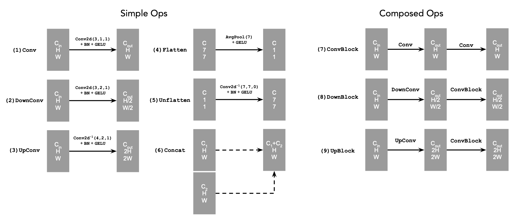
Unconditional UNet
The Unconditional UNet structure is: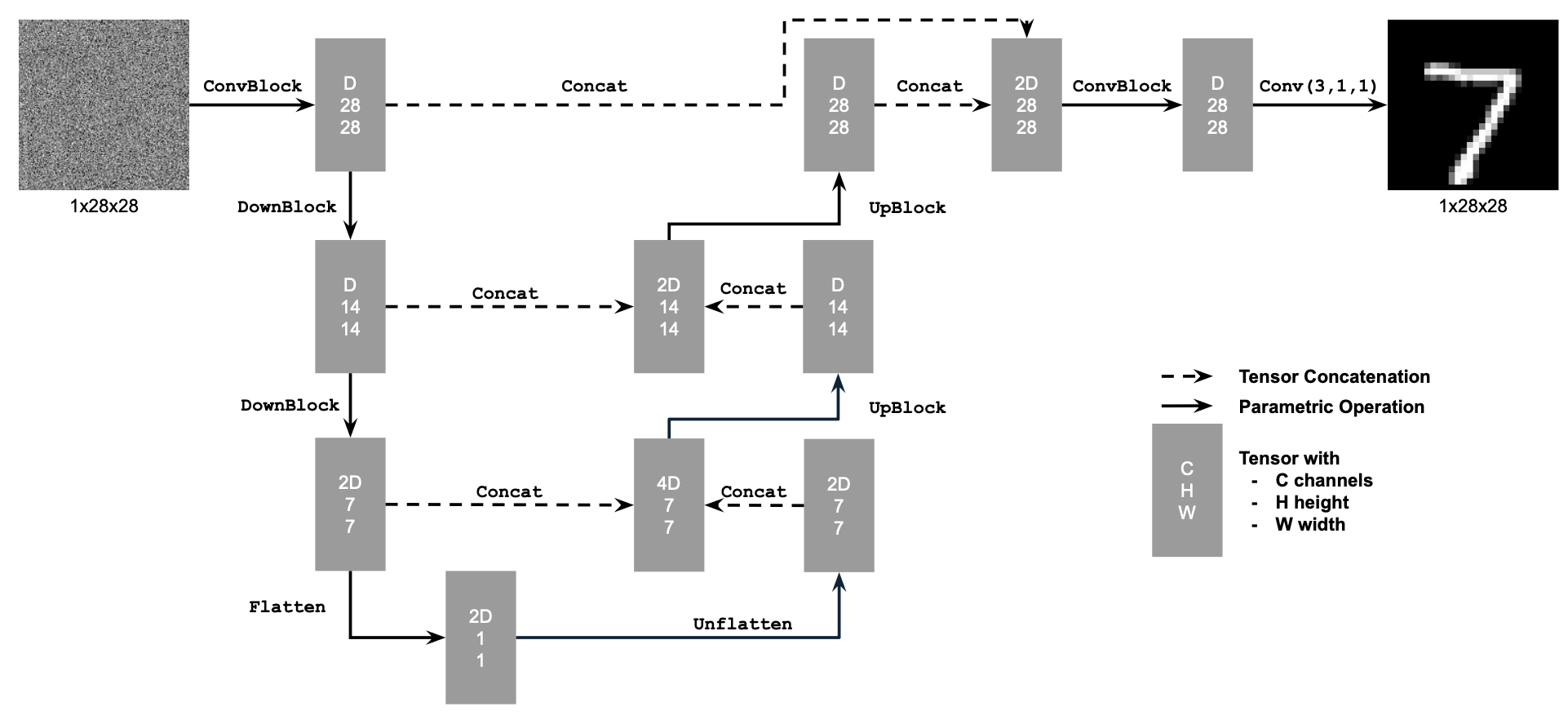
|
The number of hidden layers is $128$ for unconditional UNet.
I train the model using noisy image $z$ with $\sigma=0.5$ applied to clean images $x$. The batch size is $256$ and number of epoch is $5$. I choose Adam optimizer with initial learning rate of $1e-4$
I train the model using an L2 loss: $$L=\mathbb{E}_{z,x}\lVert D_\theta(z)-x\rVert^2$$ The training loss is:
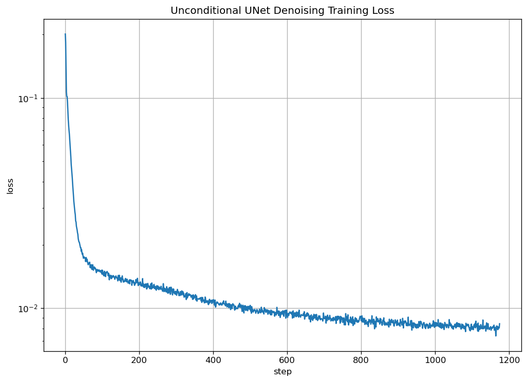
|
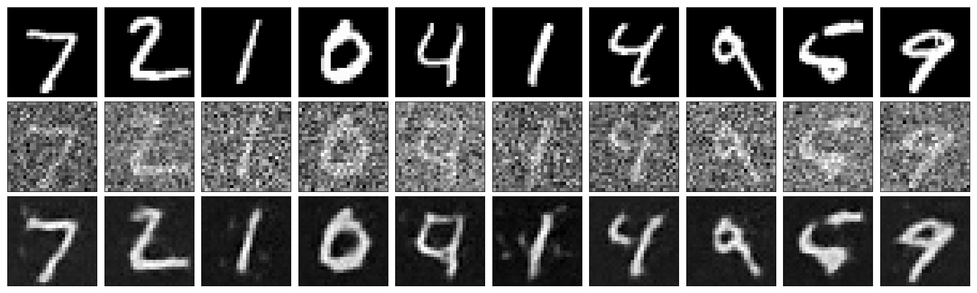
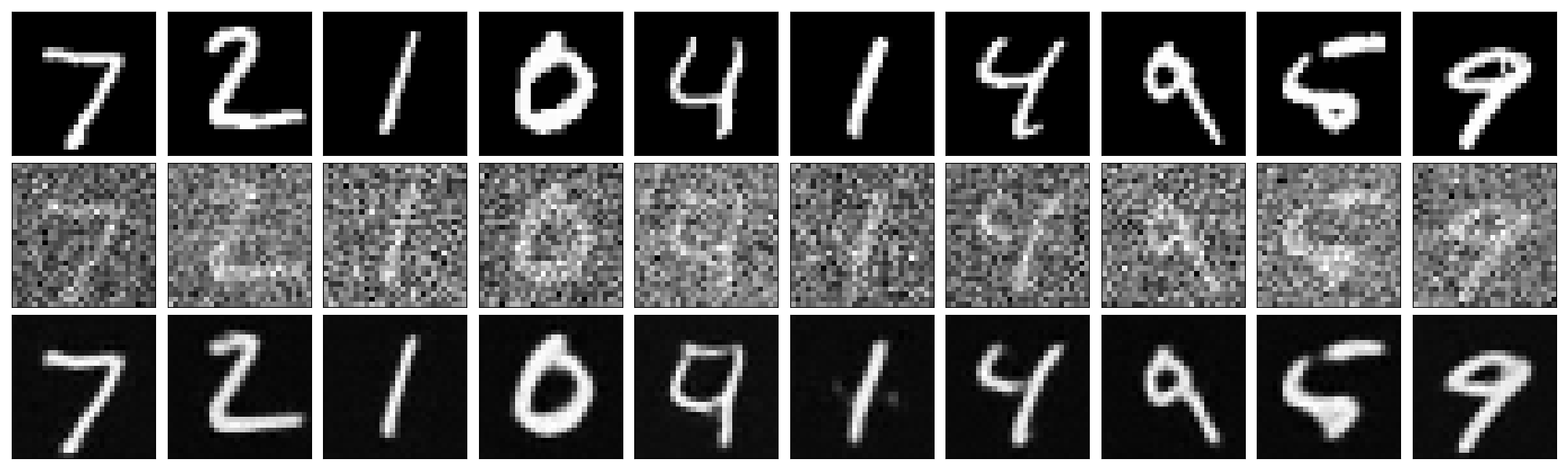
The denoise results of the training in different epoch are(top: original image, middle: noisy image, bottom: estimate original image):
|
|
I also test the model for out of distribution noise levels:
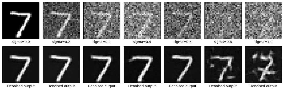
|
Time Conditional UNet
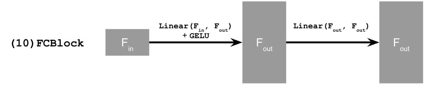
To implement a diffusion model similar to part A, I need to add the variable of time to the model to perform iteratively denoising. To do this, I added two fully connected blocks to the model by the following structure: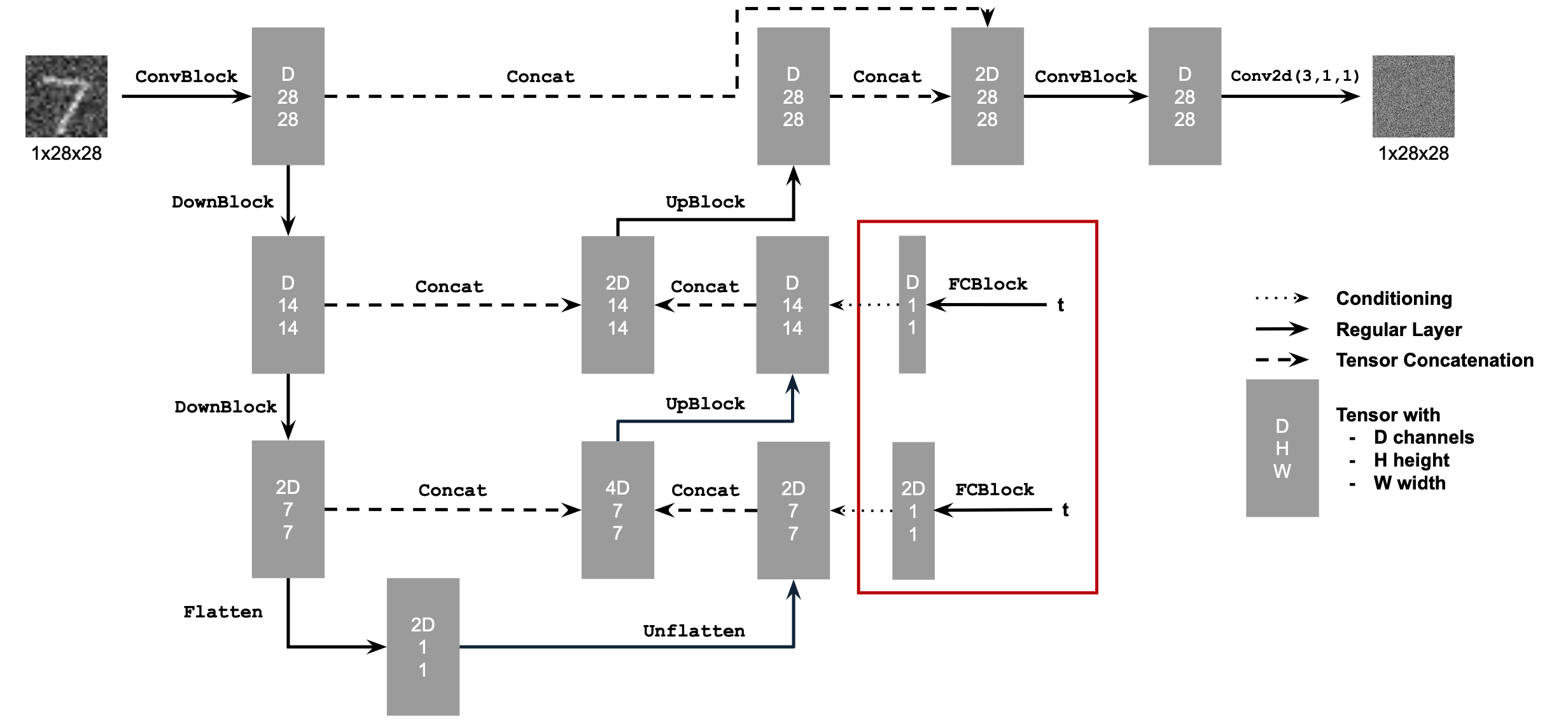
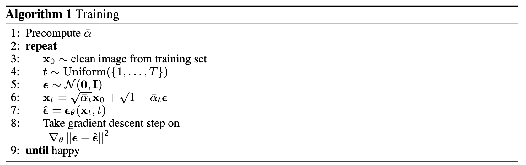
The forward process (adding noise) in this model is changed to: $$x_t = \sqrt{\bar{\alpha}_t}x_0+\sqrt{1-\bar{\alpha}_t}\epsilon\space\text{ where }\space\epsilon\sim N(0, 1)\space\text{for}\space t\in\{0,1,...,T\}$$ Some parameters are precomputed in the UNet. The computation according to DDPM paper is:
$\beta_t$: a list of $\beta$ of length $T+1$ such that $\beta_0=0.0001$ and $\beta_T=0.02$ and all other elements $\beta_t$ for $t\in\{1,...,T-1\}$ are evenly spaced between the two.
$\alpha_t$: $1-\beta_t$
$\bar{\alpha}_t$: $\prod_{s=1}^t{\alpha_s}$ is a cumulative product of $a_s$ for $s\in\{1,...,t\}$
The training algorithm of the model is:
The denoising algorithm of the model is:
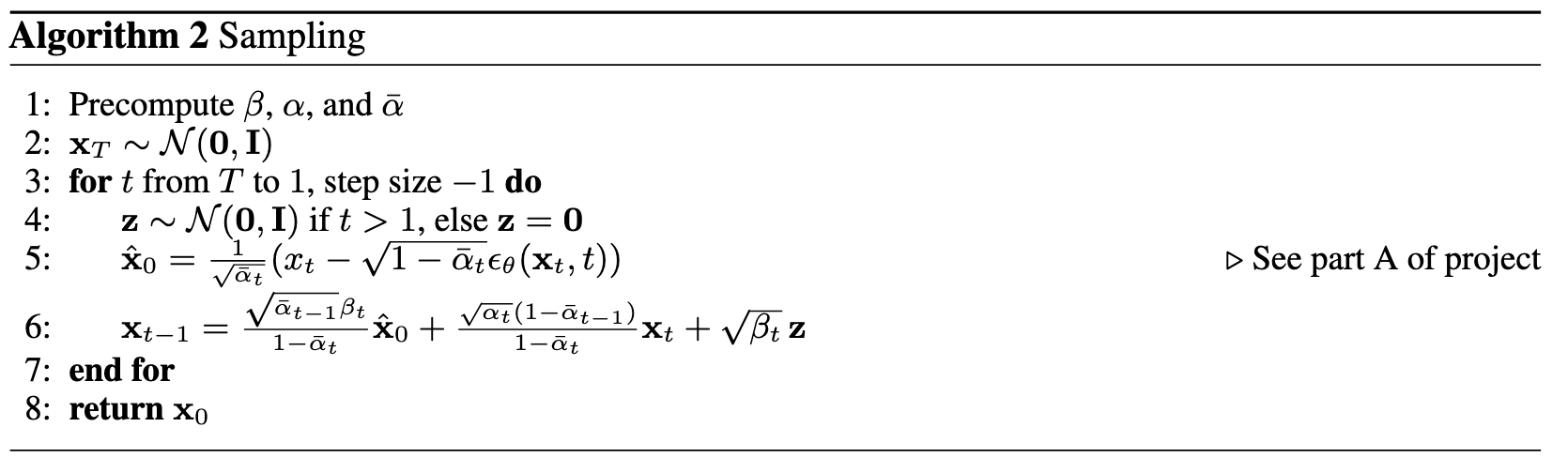
For this UNet model, the number of hidden layers is $64$. The total timestep $T=300$.
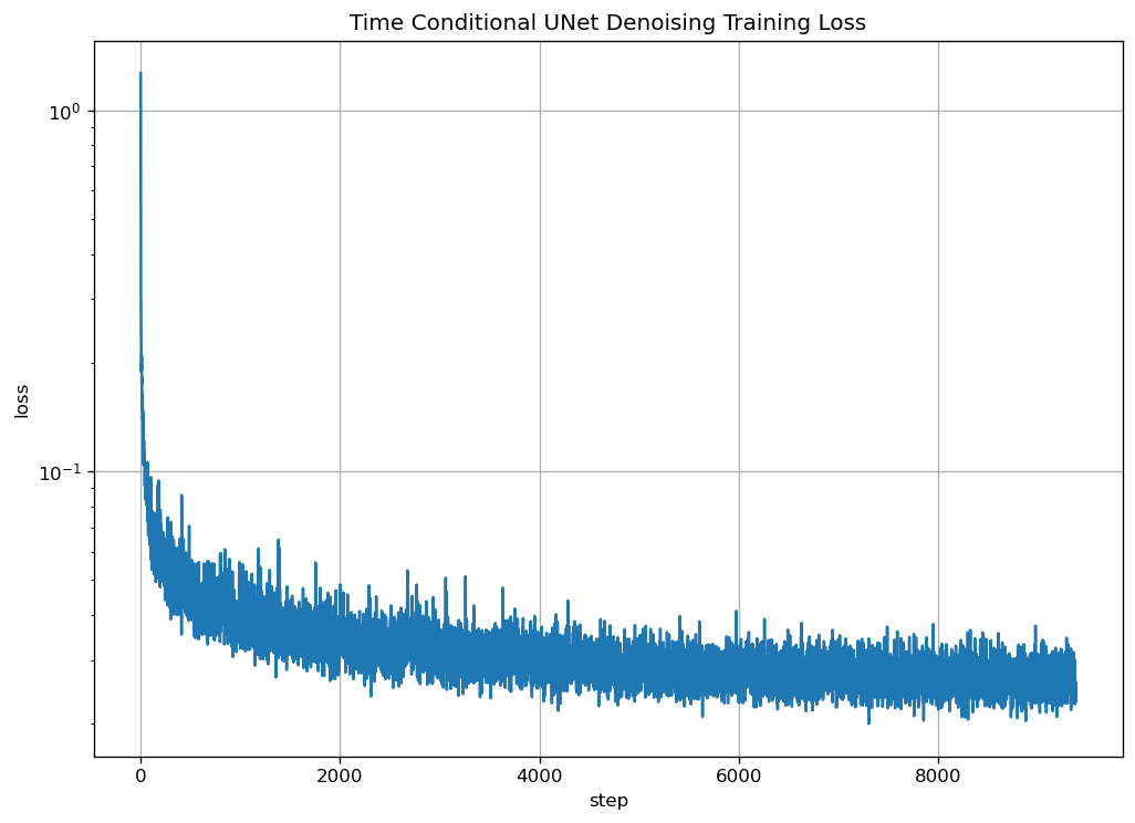
For training, I uses a batch size of $128$ and number of epoch as $20$. I still use the Adam optimizer with an initial learning rate of $1e-3$. I also set an exponential learning rate decay scheduler with a gamma of $0.1^{(1.0/\text{num_epochs})}$ by calling
torch.optim.lr_scheduler.ExponentialLR.I still use L2 loss in training: $$L=\mathbb{E}_{\epsilon, x_0,t}\lVert\epsilon_\theta(x_t,t)-\epsilon\rVert ^2$$
The training loss is:
|
The denoise results of the training in different epoch are:

|

|

|
|

|
The denoised output after training is:
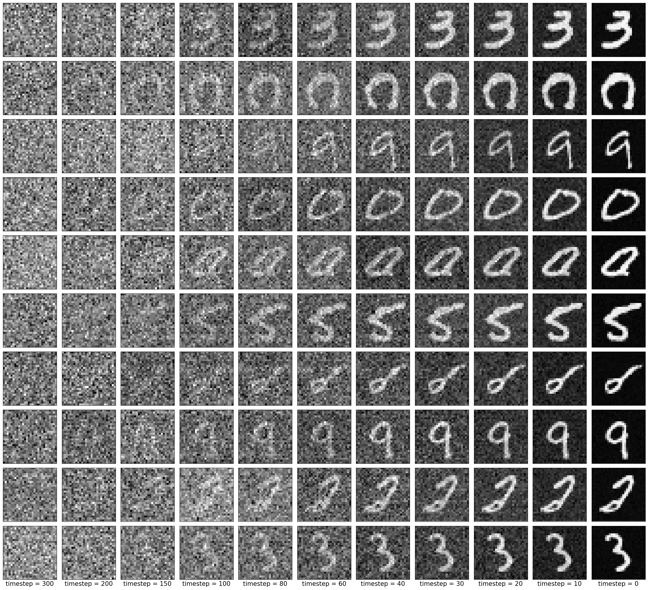
|
Class Contidional UNet
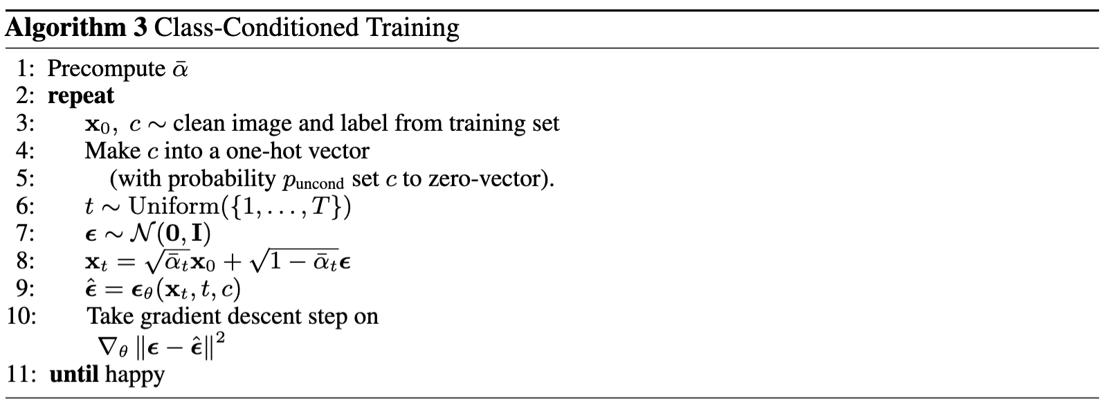
It's obvious that some of the denoised ouptput of the time conditional model is still not very good in generating digits. Hence I improve the model by adding a class condition. To implement this, I add two additional fully-connected blocks at the same places of time condition blocks.The training algorithm of the model is:
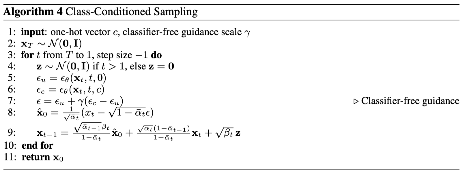
The denoising algorithm of the model is:
The model parameters and traing process are similar to the time conditional UNet model. For the class-conditioning vector $c$, I use one-hot encoding to produce the one-hot vector from the labels of the dataset. Since the UNet need to work simetimes without the class condition, I implement a dropout of class condition at a probability of $10\%$ by setting the class condition vector to 0. The training loss is:
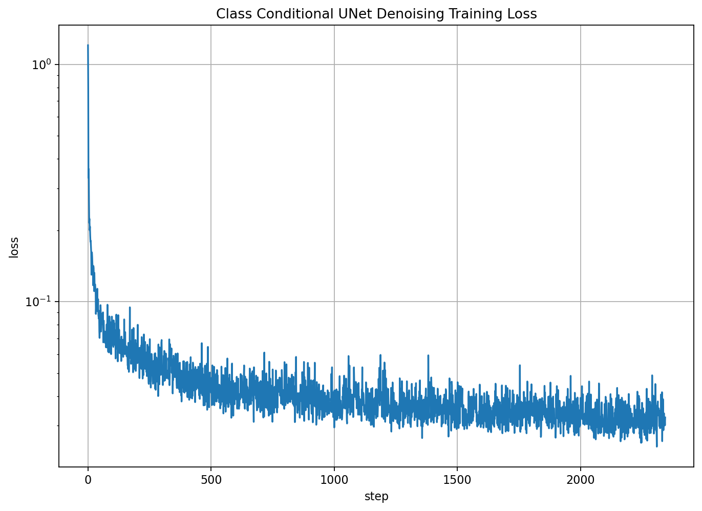
|

|

|

|

|

|
The denoised output after training is:
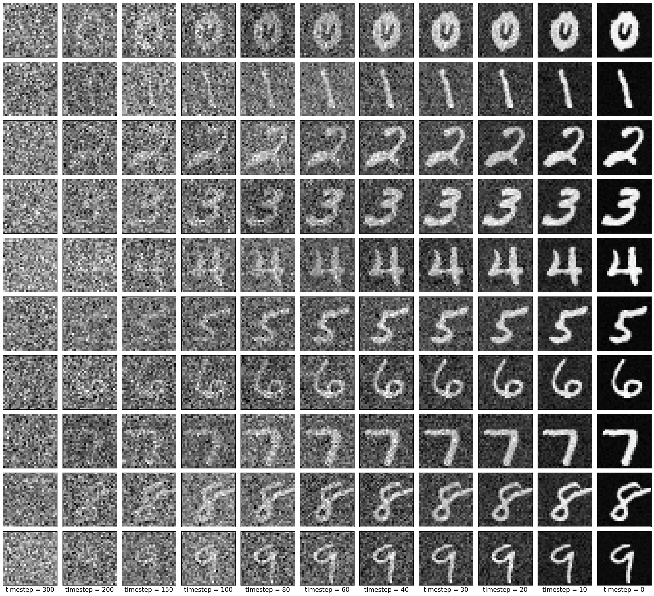
|