CS 180 Project 2: Fun with Filters and Frequencies!

Overview

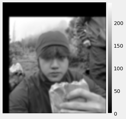
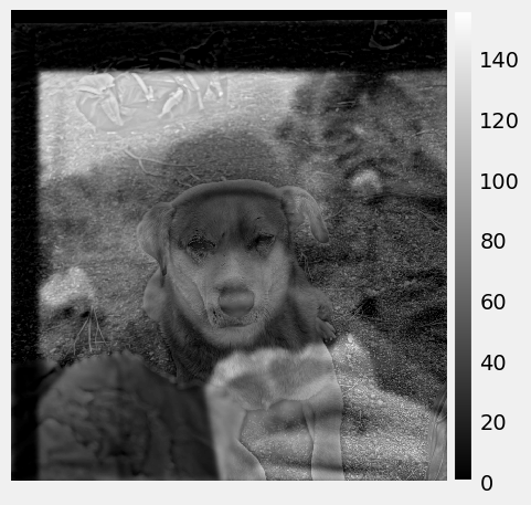
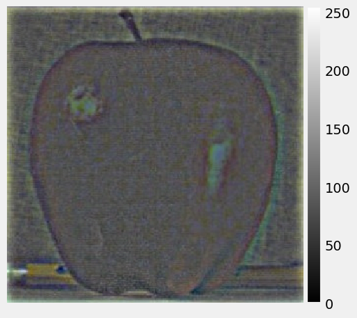
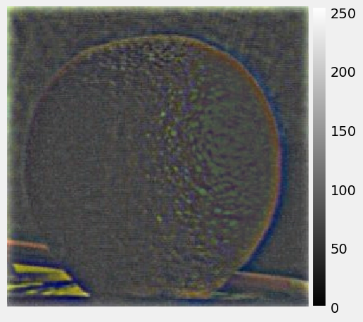
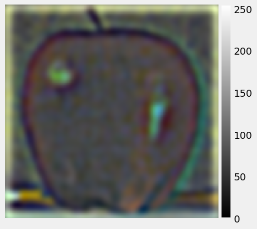
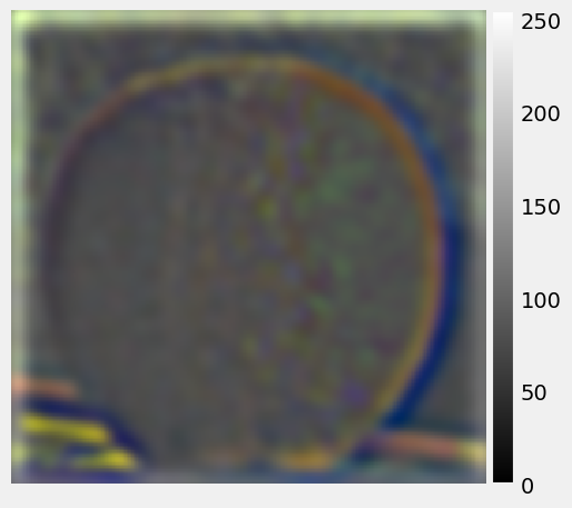
This project explores the frequency domain of images. In the first part, I built an edge detection algorithm using the Finite Derivative Operator and used the Gaussian filter to eliminate the effect of noises in edge detection. In the second part, I tried two ways of image blending. The first method blends the high and low frequencies of two images to create different impressions when looking from far and close distances. The second method used the technology called multiresolution blending introduced in the 1983 paper by Burt and Adelson. This method can create a seamless effect when blending two images with masks.

Part 1: Fun with Filters!

1.1: Finite Derivative Operator

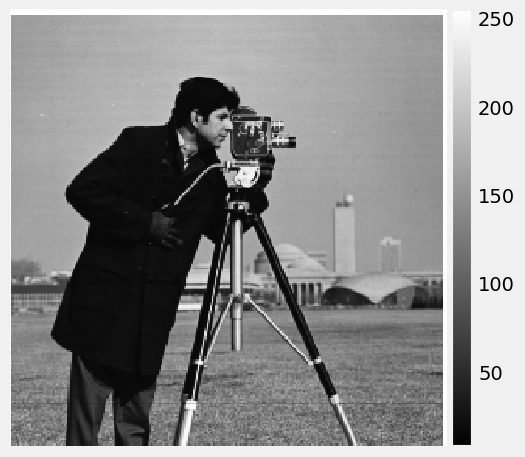
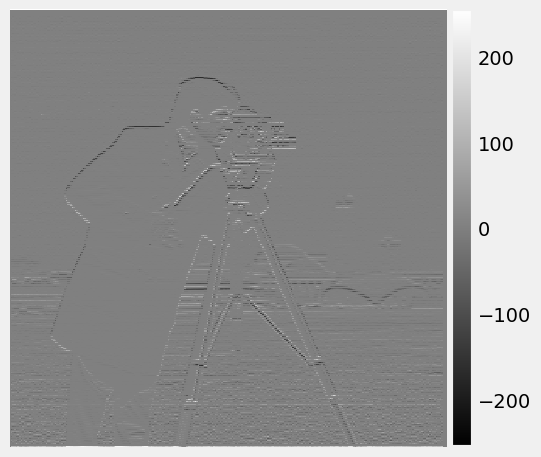
Finite derivative operator is a primitive way to detect edges. In the code, I used two simple convolution kernel to detect edges horizontally and vertically.

I used `signal.convolve2d` from the SciPy library to convolve the image with the two kernels. The result of this convolution is the gradient of the image.

Camera Man Original

Camera Man gradient dx

Camera Man gradient dy

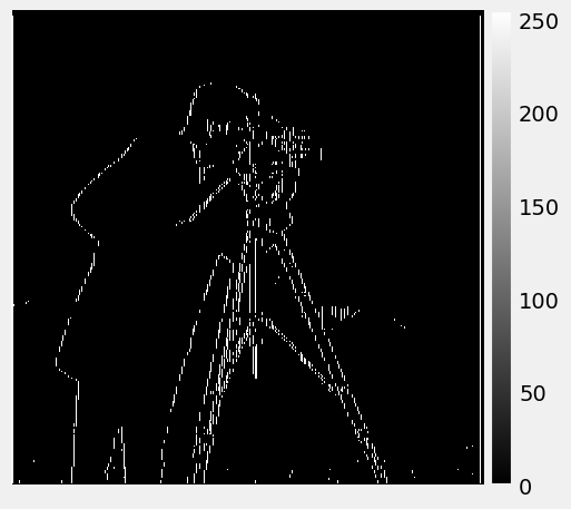
To create a better result, I binarized the gradient images to make the edges obvious. I choose a threshold of 0.25 (in range [0, 1]) so that any pixel under this value will be black and above this value will be white.

Camera Man gradient dx binarized

Camera Man gradient dy binarized

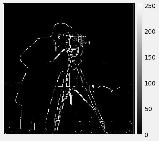
Combining the two edges using `np.sqrt(edge_imgX ** 2 + edge_imgY ** 2)` (l2 norm) can create the complete edge image:

Camera Man edge binarized

1.2: Derivative of Gaussian (DoG) Filter

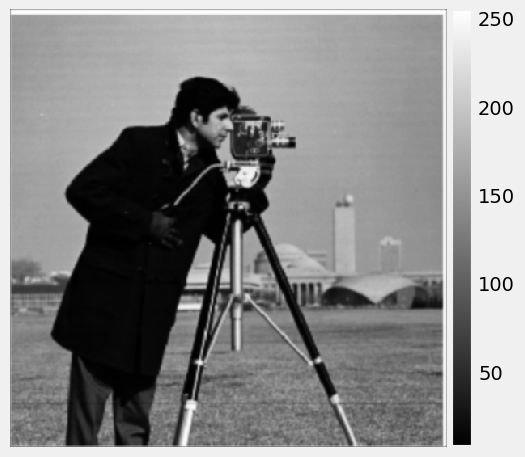
It's easy to notice that there is noise on the background. Applying a Gaussian filter can be a good way to get rid of the noise. I created the Gaussian filter by first called cv2.getGaussianKernel() to create a 1D filter. Then, I calculated the outer product of two 1d Gaussian filter to create a 2D Gaussian convolution kernel. Then I convolved the image using the Gaussian kernel. It creates blurred images that also eliminate the noise.

Camera Man Blurred

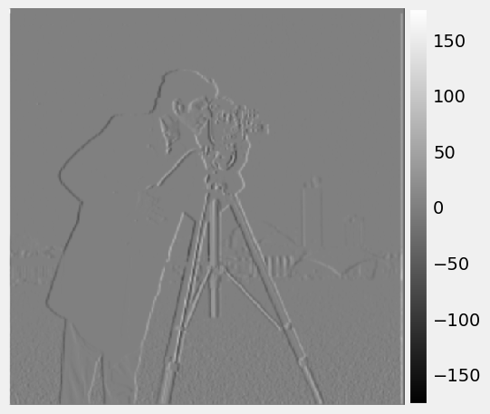
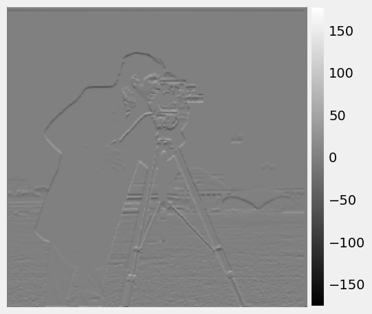
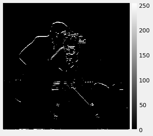
I can now take the finite derivative operator on the blurred image to achieve a better result from edge detection. We can see from the result that the detected edges are smoother and less noise.

Camera Man Blurred gradient dx

Camera Man Blurred gradient dy

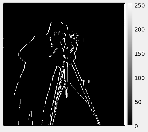
Choose 0.1 as the threshold for binarizing:

Camera Man Blurred gradient dx binarized

Camera Man Blurred gradient dy binarized

Combining the two edge images using the algorithm above creates this:

Camera Man Blurred edge

Camera Man Blurred edge binarized

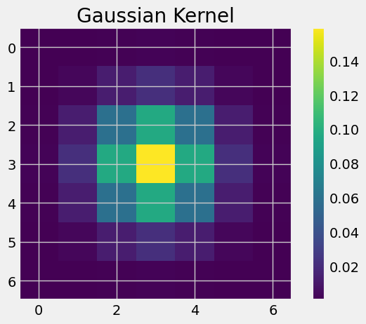
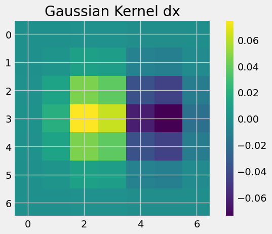
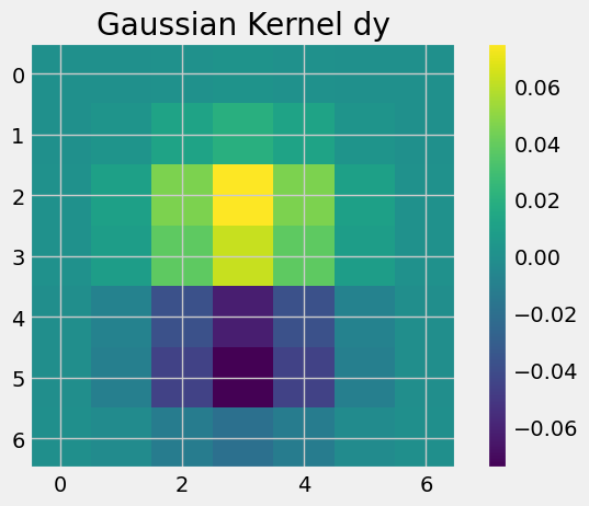
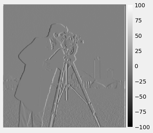
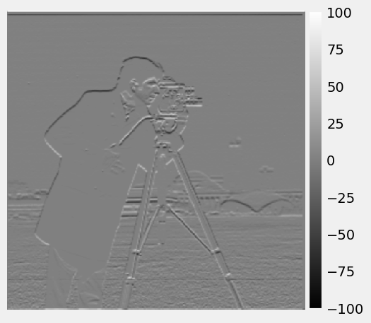
Since both applying the Gaussian filter and taking the finite derivative are linear operation, the order of the operations does not matter. I could take the finite derivative on the Gaussian filter first and then apply the derivative of Gaussian on the image.

Gaussian Kernel

Gaussian Kernel dx

Gaussian Kernel dy

Camera Man Gaussian dx

Camera Man Gaussian dy

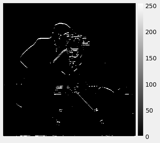
Still choose 0.1 as the threshold for binarizing:

Camera Man Gaussian dx binarized

Camera Man Gaussian dy binarized

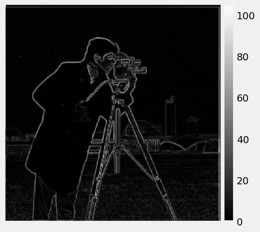
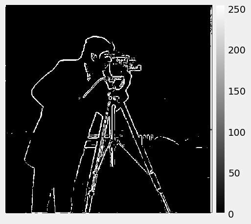
Combining the two edge images using the algorithm above creates this:

Camera Man Gaussian dx binarized

Camera Man Gaussian dy binarized

We can see either ways create mostly identical results except for some minor differences. The two binarized images are exactly the same under the same threshold. This is becasue finite derivative and Gaussian filter are both linear process. Hence the order of the two manipulation does not matter.

Gaussian then Derivative

Derivative of Gaussian

Part 2: Fun with Frequencies!

2.1 Image Sharpening

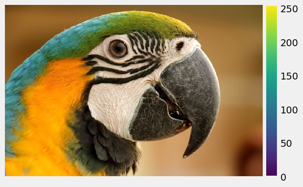
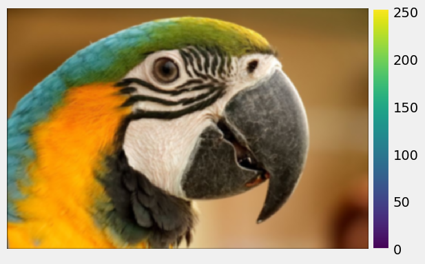
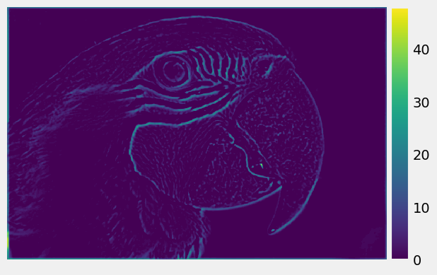
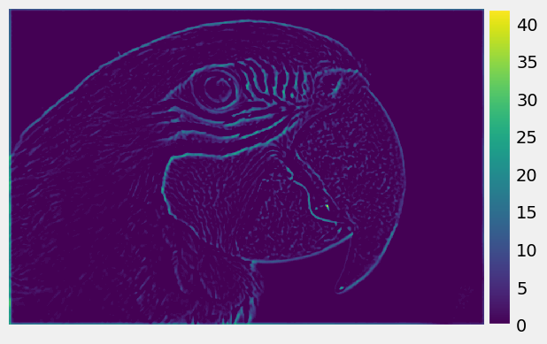
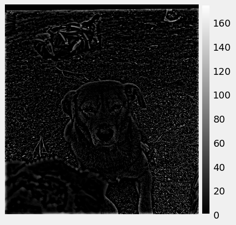
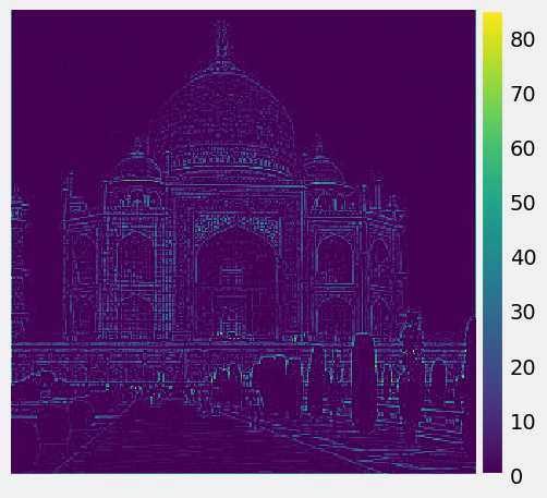
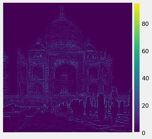
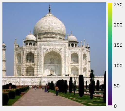
The idea of image sharpening is to add more high frequency content to the image. Adding high frequency content can make the image look like having more details. To extract the high frequency content, we first create a blurred version of the image (represent to low frequency part). Then we subtract the original image with the blurred image. Finally, we could add the extracted high frequency content to the original image to create a sharpen image.

High frequency of the R, G, B channels of Taj:

High frequency of R channel

High frequency of G channel

High frequency of B channel

Adding high frequency to the original image:

Taj Original

Taj Sharpen

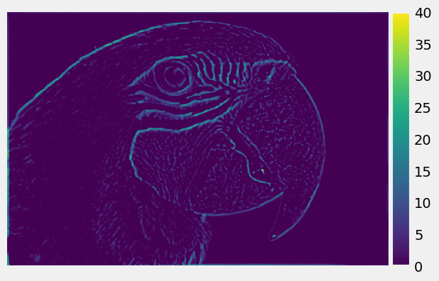
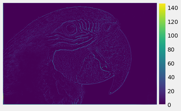
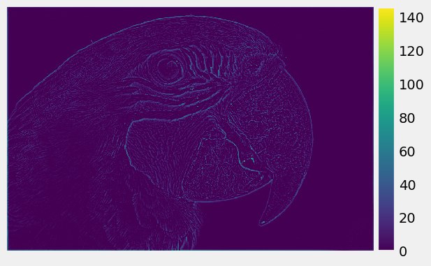
High frequency of the R, G, B channels of Parrot:

High frequency of R channel

High frequency of G channel

High frequency of B channel

I then blur the image first and try sharpen the image to recover its initial status.

The result shows that although sharpening the blurred image can make it looks sharper than the blurred one. However, it's still pretty obvious that it lacks some details compare to the original image. The lost information cannot be recovered by image sharpening.

2.2 Hybrid Images

This part of the project is to create hybrid images using the method introduced in the paper published in the SIGGRAPH 2006 by Oliva, Torralba, and Schyns. The key idea is to merge the high frequency of one image and the low frequency of another image. When looking close to the image, the high frequency part is clear, thus look like the first image. However, when looking in a far distance, we can only see the low frequency part, so it looks like the second image.

My approach is still use the Gaussian filter to get the low frequency part of an image. Then use the original image minus the low frequency part to get the high frequency part.

In Nutmeg and Derek's example, I will create an image using the high frequency of Nutmeg and low frequency of Derek.

Diving into the frequency domain, the algorithm works successfully on extracting the high and low frequencies. From Nutmeg's high frequency image, the high frequency part is enhanced and low frequency part is reduced. In the Derek Low Frequency's frequency domain, only low frequencies are left in the image.

In the next example, I blended me with a dog I don't know the name who trying to steal my food.

2.3 Gaussian and Laplacian Stack

A image stack is a group of images with the same resolution. However, filters are applied to different layer of stack.

To create a Laplacian Stack, I need to first create a Gaussian stack. The Gaussian stack implementation is simply taking the original image as the first layer and applying the Gaussian filter on the previous layer as the next layer. Then for the Laplacian stack, each layer will be the same layer of the Gaussian stack minus the next layer of the Gaussian stack. For the last layer of the Laplacian stack, it just uses the same image as the last layer of the Gaussian stack.

2.4 Multiresolution Blending

The key point of the multiresolution blending is to blend different frequency with differnt masks to create a seamless effect. The approach first crate a Gaussian stack for the mask and Laplacian stacks for two images that are going to stack. After that, for each layer of the stack, the algorithm blends them using `blended_img = (1 - mask) * img1 + mask * img2`. As a result, different frequencies are blended with suitable masks.

The oraple is blended from an apple image and an orange image from the previous part.

I find a set of images collected by Pablo Rochat interesting. I decided to blend some images from his photo collection

Nutmeg Low Frequency with Gaussian sigma 10	Nutmeg High Frequency _	Derek Low Frequency with Gaussian sigma 13
Nutmeg Low Frequency Frequency Domain	Nutmeg High Frequency Frequency Domain	Derek Low Frequency Frequency Domain

Slipper	Fish
Mask	Fishliper

Sunglasses	Sauce
Mask	Sauceglasses